Patent application title: Method for optimizing inequality and equality constrained resources allocation problems in industrial applications
Inventors:
Phil Kongtcheu (Jersey City, NJ, US)
IPC8 Class: AG06F1518FI
USPC Class:
706 19
Class name: Neural network learning task constraint optimization problem solving
Publication date: 2009-12-03
Patent application number: 20090299928
Inventors list |
Agents list |
Assignees list |
List by place |
Classification tree browser |
Top 100 Inventors |
Top 100 Agents |
Top 100 Assignees |
Usenet FAQ Index |
Documents |
Other FAQs |
Patent application title: Method for optimizing inequality and equality constrained resources allocation problems in industrial applications
Inventors:
Phil Kongtcheu
Agents:
PHIL KONGTCHEU;PFK TECHNOLOGIES
Assignees:
Origin: JERSEY CITY, NJ US
IPC8 Class: AG06F1518FI
USPC Class:
706 19
Patent application number: 20090299928
Abstract:
In industrial applications, the invention relates to various algorithms
for determining optimal resources or assets allocations under various
equality and inequality constraints. In particular, constrained quadratic
or conic optimization problems of unique importance for portfolio asset
allocation are seamlessly solved in analytic and efficient ways. In
addition, by providing exact or analytic optimum expressions, robustness
can be readily ascertained.Claims:
1. In industrial applications problems, a method for deriving the one or
more local extrema of an optimization problem, said method comprising the
steps of:Deriving the KKT equations and inequalities,Solving the KKT
equations by:a) Establishing a system of block-coordinate decomposition
to facilitate incremental consideration of additional constraints;b)
starting from the lesser applicable number of inequality constrained
local extrema in a list indexing potential KKT local extrema, iteratively
considering the cases where additional inequality boundaries are
reached;c) facilitate equations resolution by assigning to the slacking
parameters corresponding to inequality constraints not reached the value
zero;d) using an exact or approximate method to derivei) Wq the one
or more vector of coordinates that are not supposed to have reached the
inequality boundaries andii) γp the one or more vector of KKT
slacking parameters corresponding to coordinates that are supposed to
have reached the equalities boundaries.
2. The method of claim 1, where any computed candidate local extremum Wq is excluded from a list of acceptable local extrema if any one in either of the two groups of KKT inequalities is not verified:i) the inequality constraints involving the candidate extremum vector W and its coordinates Wq;ii) the sign constraints involving the slacking parameters vector γp;
3. The method of claim 1, where equality constrains and the selected inequality reached at the boundary for the given extremum result in an empty set, said method triggering the elimination of a priori subsequent descendent cases corresponding to additional constraints from a list of admissible local extrema.
4. The method of claim 1, where the candidate local extrema is excluded from an a priori list of admissible local extrema if the second order derivative or the Hessian isi) not symmetric positive semi-definite for a minimum orii) not symmetric negative semi-definite for a maximum.
5. The method of claim 4 where a priori subsequent descendent cases corresponding to additional constraints are eliminated from a list of admissible local extrema if it can be deduced such dependent cases may not verify second order derivative conditions.
6. The method of either of claim 2, 3, 4 where a local extrema verifying all admissibility conditions triggers the elimination of a priori subsequent descendent cases corresponding to additional constraints from a list of admissible local extrema.
7. The method of claim 5, where deducing that dependent cases may not verify second order derivative conditions or handling linear inequality constraints is facilitated by a change of variables.
8. The method of claim 1, where the target or the constraints are linear or quadratic or contain unit step discontinuities, said method resulting in an exact analytic method to derive Wq or γp.
9. The method of claim 1, where a priory subsequent descendent cases corresponding to additional constraints in a list of admissible local extrema are grouped together for evaluation in order to reduce the total computational cost.
10. The method of claim of claim 8, where second order derivative conditions are trivially verified, said method reducing the computational cost on computing the inverse of the Hessian through a computationally inexpensive relationship with the inverse of a parent Hessian.
11. The method of claim 1, said method facilitating dimension reduction through permutations invariance or other similar dimension reducing transformations.
12. In industrial applications problems a method for deriving the one or more global extrema of an optimization problem, said method comprising the steps ofi) establishing a list of admissible local extremaii) iteratively comparing among said local extrema and progressively eliminating suboptimal candidates
13. The method of either of claim 8 or 12, said method facilitating parametric sensitivity analysis by differentiating the expression of extrema with respect to desired parameters.
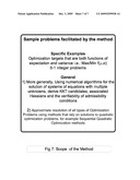
14. The method of claim 8, said method facilitating the resolution of an optimization problem that is a function of expectation and variance, said method comprising the steps of:i) solving the optimization on an expectation target for a fixed variance;ii) using the analytic expression of the local extrema to find the fixed variance which optimizes the function of expectation and variance;iii) replacing said optimal variance in the fixed variance of step i).
15. The method of claim 8, said method facilitating the resolution of an optimization problem that is a function of expectation and variance, said method comprising the steps of:i) solving the optimization on a variance target for a fixed expectation;ii) using the analytic expression of the local extrema to find the fixed expectation which optimizes the function of expectation and variance;iii) replacing said optimal expectation in the fixed variance of step i).
16. The method of claim 8, said method facilitating a general function optimization problem that is decomposed into sequences of quadratic optimization problems.
17. In industrial applications such as in financial markets, a method for establishing an optimal VAR fund, an optimal Sharpe Ratio fund or an optimal Kelly criterion fund, said method including the steps of:i) establishing the assets in which the fund can invest in and a method to derive their expected returns and covariance matrix;ii) specifying boundaries on allocation in each asset;iii) choosing a VAR strategy and specifying the maximum value at risk given a specified confidence level, or choosing a Sharpe Ratio strategy or Kelly criterion strategy;iv) if choosing a VAR strategy, transforming the Value at Risk boundary number into a variance number via distributional information or the Chebyshev inequality;v) solving the optimization problem to obtain the optimal asset allocations.
Description:
BACKGROUND OF THE INVENTION
[0001]In industrial applications, a substantial number of problems of efficient allocations of resources can be translated into the mathematical resolution of one or more constrained optimization problems, that is problems in which one seeks to minimize or maximize a real function by systematically choosing the values of real or integer variables from within a constrained allowed set.
[0002]As a subset of optimization problems, quadratic or conic optimization problems comprise one of the most important areas of nonlinear programming. They are currently solved in practical applications preferentially using variations of so-called "interior point methods"i that are generally relevant for convex optimization problems. Numerous practical problems, including problems in financial portfolio optimization, portfolio hedging, planning and scheduling, economies of scale, and engineering design, and control are naturally expressed as quadratic optimization problems. i"Numerical Optimization Second Edition" Nocedal & Wright Springer Series in Operations Research, 2006
[0003]We describe a new and more effective method for solving optimization problems in general by actually explicitly solving the apparently intractable Karush-Kuhn Tucker (KKT) equations and inequalities associated with the mathematical formulation of the problems. The general method outlined in our drawings and below is illustrated in detail through the resolution of classical quadratic and conic optimization problems.
BRIEF DESCRIPTION OF THE SEVERAL VIEWS OF THE DRAWINGS
[0004]FIG. 1 illustrates the components and structure of the algorithm implementing our method.
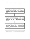
[0005]FIG. 2 describes the procedure for obtaining candidate local extrema from KKT equations.
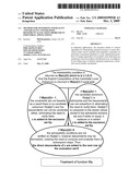
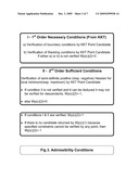
[0006]FIG. 3 outlines the conditions under which a local extremum may be admissible via the verification of first and second order inequality constraints.
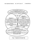
[0007]FIG. 4 outline the disposition of potential candidate local extrema.
[0008]FIG. 5 describes various strategies that may be used to effect computational gains.
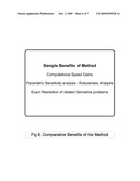
[0009]FIG. 6 summarizes obvious benefits of the method.
[0010]FIG. 7 expands on the scope of applications.
DETAILED DESCRIPTION
[0011]FIGS. 1 to 7 present the method in general. Our detailed description provides added clarity through the detailed study of two specific cases. These illustrations are made even more practical in the Mathematica computer implementation of Appendix 2.
[0012]Case 1: A Generic Quadratically Constrained Minimization Problem
[0013]This problem can be generally stated analytically as:
[0014]Find the solution to the constrained quadratic optimization problem
Min 1 2 W t Σ W + C t W subject to constraints ##EQU00001## { AW t - B = 0 ; W - M _ + M _ 2 ≦ M _ - M _ 2 with M _ , W , C , M _ .di-elect cons. m , M _ ≦ W ≦ M _ , A .di-elect cons. s × m ; Rank ( A ) = s ≦ m , B .di-elect cons. s ##EQU00001.2##
[0015]Solution:
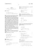
[0016]We proceed as outlined in FIG. 2. The KKT Equations are:
K = 1 2 W t Σ W + C t W + λ ' t ( AW - B ) - γ - ( W - M _ ) + γ + ( W - M _ ) λ ' .di-elect cons. s , M _ ≦ W ≦ M _ , A .di-elect cons. s × m ; ##EQU00002##
the so-called slacking parameters γ.sup.+,γ.sup.- must verify γ.sup.+,γ.sup.-.di-elect cons..sub.+m,
[0017]We note γ.sup±gamma..sup.-; We have:
{ ∇ K t = Σ W + C + A t λ ' + γ = 0 ( 1 ) AW - B = 0 ( 2 ) γ + ( W - M _ ) = 0 , γ - ( W - M _ ) = 0 ( 3 ) ∇ K t = Σ W + C + A t λ ' + γ = 0 ( 1 ) ##EQU00003##
[0018]We suppose there are p active constraints and q=m-p non-active ones. We perform a block decomposition along active and non active constraints. We introduce the operator LinSol defined in Appendix 1.
[0019]The non-active constraints lead to γq=0. Hence,
( 1 ) ⇄ - ( s pp s pq s pq t s qq ) ( M p W q ) = ( A p t λ ' A q t λ ' ) + ( C p C q ) + ( γ p 0 ) ##EQU00004## ( 1 ) ⇄ - ( s pp s pq s pq t s qq ) ( M p W q ) = ( A p t λ ' A q t λ ' ) + ( C p C q ) + ( γ p 0 ) ##EQU00004.2## W q = - LinSol ( s qq , s pq t M p + A q t λ ' + C q ) ; ##EQU00004.3## γ p = - s pp M p - A p t λ ' - C p + s pq LinSol ( s qq , s pq t M p + A q t λ ' + C q ) ; ##EQU00004.4## ( 2 ) ⇄ ( A p A q ) ( M p W q ) - B = 0 ##EQU00004.5##
[0020]Note that Ap is an s×p matrix and Aq is an s×q matrix.
( 2 ) ⇄ A q W q = B - A p M p ; ##EQU00005## ( 1 ) + ( 2 ) - A q LinSol ( s qq , s pq t M p + A q t λ ' + C q ) = B - A p M p ##EQU00005.2## A q LinSol ( s qq , A q t ) λ ' = A p M p - B - A q LinSol ( s qq , s pq t M p + C q ) ##EQU00005.3## λ ' = LinSol ( A q LinSol ( s qq , A q t ) , A p M p - B - A q LinSol ( s qq , s pq t M p + C q ) ) ##EQU00005.4##
[0021]We recall
W q = - LinSol ( s qq , s pq t M p + A q t λ ' + C q ) ; γ p = - s pp M p - A p t λ ' - C p + s pq LinSol ( s qq , s pq t M p + A q t λ ' + C q ) ; ##EQU00006##
[0022]This provides the general expression of the KKT local minima. In order for them to be admissible, they have to verify the admissibility conditions outlined in FIG. 3.
[0023]Appendix 2 shows how the algorithm implementing the structure outlined in FIG. 1 disposes of the local extrema as shown in FIG. 4. and implements the applicable strategies to effect computational gains as described in FIG. 5. The computer code in Appendix 2 is written in Mathematica, owned and copyrighted by Wolfram research. For clarity purposes, the matrix Σ is assumed to be symmetric positive definite. This algorithm also counts the number of cases of local extrema actually computed to measure the effectiveness of the computational strategies used. It empirically appears that the number of local extrema actually computed, which a priory grows exponentially with m, becomes here reduce to polynomial of order approximating 3, supporting our claims of computational gains outline in FIG. 6.
[0024]Case 2: A Maximization Problem with Quadratically Constrained Equations and Inequalities
[0025]This case illustrate that the constraints may be linear or quadratic. It is typically classified as a conic optimization problem. It may be used to solve a broad number of assets allocations problems in finance.
[0026]Problem
[0027]This problem can be generally stated analytically as finding the solution to the constrained quadratic optimization problem:
[0028]MaxWtR subject to constraints
{ AW - B = 0 ; W t Σ W - σ 2 = 0 W - M _ + M _ 2 ≦ M _ - M _ 2 with M _ , W , M _ , R .di-elect cons. m , M _ ≦ W ≦ M _ , σ .di-elect cons. + , A .di-elect cons. s × m ; Rank ( A ) = s ≦ m , B .di-elect cons. s ##EQU00007##
[0029]Solution:
[0030]The KKT Equations are:
K = W t R + λ ' t ( AW - B ) + λ 2 ( W t Σ W - σ 2 ) - γ - ( W - M _ ) + γ + ( W - M _ ) λ ' .di-elect cons. s , λ .di-elect cons. , M _ ≦ W ≦ M _ .di-elect cons. m , A .di-elect cons. s × m ; ##EQU00008## Rank ( A ) = s ≦ m , B .di-elect cons. s ##EQU00008.2##
[0031]The so-called slacking parameters γ.sup.+,γ.sup.- must verify γ.sup.+,γ.sup.- .sub.+m,
[0032]We note γ.sup±gamma..sup.-; We have:
( I ) { ∇ K = R t + λ ' t A + λ W t Σ + γ t = 0 ( 1 ) AW - B = 0 ( 2 ) W t Σ W - σ 2 = 0 ( 3 ) γ + ( W - M _ ) = 0 , γ - ( W - M _ ) = 0 ( 4 ) ##EQU00009##
[0033](i) Let's first deal with constraints (1)
[0034]We suppose there are p active constraints, 0≦p≦m, q=m-p.
[0035]We note according to a block matrix decomposition
Σ = ( s pp s pq s pq t s qq ) ; ##EQU00010## = ( 1 0 0 m t ) = ( pp 0 pq 0 qp 0 qq ) ; ##EQU00010.2## i .di-elect cons. { - 1 , 0 , 1 } , ##EQU00010.3##
where spp,spq,sqq,εpp are block matrices with the indices indicating the number of rows and columns respectively.
[0036]We also note
γ = ( γ p 0 ) ; R = ( R p R q ) ; ##EQU00011## W = ( 1 2 ( M _ p + M _ p ) + pp 2 ( M _ p + M _ p ) M p W q ) ; ##EQU00011.2##
[0037]Expression of Wq, γp
( ∇ K t ) t = R + A t λ ' + λ Σ W + γ = 0 - λ Σ W = R + A t λ ' + γ - λ ( s pp s pq s pq t s qq ) ( M p W q ) = ( R p R q ) + ( A p t λ ' A q t λ ' ) + ( γ p 0 ) { γ p = λ ( s pq s qq - 1 s pq t - s pp ) M p + ( s pq s qq - 1 ( R q + A q t λ ' ) - ( R p + A p t λ ' ) ) W q = - s qq - 1 ( s pq t M p + 1 λ ( R q + A q t λ ' ) ) ( 1 ) ##EQU00012##
[0038]Elimination of λ'
(2)AqWq=B-ApMp
[0039]Note that Ap is an s×p matrix and Aq is an s×q matrix.
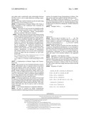
( 1 ) + ( 2 ) - A q s qq - 1 ( s pq t M p + 1 λ ( R q + A q t λ ' ) ) = B - A p M p ##EQU00013## ( A p - A q s qq - 1 s pq t ) M p - B = 1 λ A q s qq - 1 R q + 1 λ A q s qq - 1 A q t λ ' ; χ s A q s qq - 1 A q t ; ##EQU00013.2## λ ' = χ s - 1 ( λ ( ( A p - A q s qq - 1 s pq t ) M p - B ) - A q s qq - 1 R q ) ; ##EQU00013.3## 1 λ ( R q + A q t λ ' ) = 1 λ ( R q + A q t χ s - 1 ( λ ( ( A p - A q s qq - 1 s pq t ) M p - B ) - A q s qq - 1 R q ) ) ; ##EQU00013.4## 1 λ ( R q + A q t λ ' ) = A q t χ s - 1 ( ( A p - A q s qq - 1 s pq t ) M p - B ) + 1 λ ( I q - A q t χ s - 1 A q s qq - 1 ) R q ; ##EQU00013.5## W q = - s qq - 1 ( s pq t M p + A q t χ s - 1 ( ( A p - A q s qq - 1 s pq t ) M p - B ) + 1 λ ( I q - A q t χ s - 1 A q s qq - 1 ) R q ) ##EQU00013.6## γ p = λ ( s pq s qq - 1 s pq t - s pp ) M p + ( s pq s qq - 1 ( R q + A q t λ ' ) - ( R p + A p t λ ' ) ) ##EQU00013.7## γ p = λ ( ( s pq s qq - 1 s pq t - s pp + ( s pq s qq - 1 A q t - A p t ) χ s - 1 ( A p - A q s qq - 1 s pq t ) ) M p - ( s pq s qq - 1 A q t - A p t ) χ s - 1 B ) + ( s pq s qq - 1 R q - R p ) - ( s pq s qq - 1 A q t - A p t ) χ s - 1 A q s qq - 1 R q ##EQU00013.8##
[0040]Elimination of λ
W q = 1 λ a q - b q ; W = ( M p W q ) = 1 λ ( 0 a q ) + ( M p - b q ) ; a ( 0 a q ) ; b ( M p - b q ) ; W = 1 λ a - b ; a = ( 0 - s qq - 1 ( I q - A q t χ s - 1 A q s qq - 1 ) R q ) ; b = ( - I p s qq - 1 ( s pq t + A q t χ s - 1 ( A p - A q s qq - 1 s pq t ) ) ) M p - ( 0 p s qq - 1 A q t χ s - 1 B ) ; W t Σ W = ( 1 λ a - b ) t Σ ( 1 λ a - b ) = 1 λ 2 a t Σ a - 2 a t Σ b 1 λ + b t Σ b W t Σ W - σ 2 = 0 1 λ 2 a t Σ a - 2 a t Σ b 1 λ + b t Σ b - σ 2 = 0 ; If σ 2 ≧ ( a t Σ a ) ( b t Σ b ) - ( a t Σ b ) 2 a t Σ a , 1 λ ± = a t Σ b a t Σ a ± 1 a t Σ a ( σ 2 - ( a t Σ a ) ( b t Σ b ) - ( a t Σ b ) 2 a t Σ a ) W ± = 1 λ ± a - b = ( a t Σ b a t Σ a a - b ) ± 1 a t Σ a ( σ 2 - ( a t Σ a ) ( b t Σ b ) - ( a t Σ b ) 2 a t Σ a ) a R t ( W - - W + ) = - 2 1 a t Σ a ( σ 2 - ( a t Σ a ) ( b t Σ b ) - ( a t Σ b ) 2 a t Σ a ) R t a ( 3 ) ##EQU00014##
[0041]Note that sqq-1(Iq-Aqtχs-1Aqsqq.su- p.-1) is a symmetric positive semi-definite matrix.
R t ( W - - W + ) = - 2 1 a t Σ a ( σ 2 - ( a t Σ a ) ( b t Σ b ) - ( a t Σ b ) 2 a t Σ a ) R t a ##EQU00015## Hence = 2 1 a t Σ a ( σ 2 - ( a t Σ a ) ( b t Σ b ) - ( a t Σ b ) 2 a t Σ a ) ( R q ) t ( s qq - 1 ( I q - A q t χ s - 1 A q s qq - 1 ) ) R q ≧ 0 ##EQU00015.2##
[0042]Therefore,
W = W - = ( a i Σ b a i Σ a - 1 a t Σ a ( σ 2 - ( a t Σ a ) ( b t Σ b ) - ( a t Σ b ) 2 a t Σ a ) ) a - b ##EQU00016##
[0043]The sufficient second order condition for a maximum translates as
1 λ ≦ 0 , ##EQU00017##
i.e.:
(btΣb-σ2)≦0 or atΣb≦0
[0044]Once we have the general formula for candidate local optimum here, the treatment to obtain the global maximum mirrors Case 1. This case can be extended in a variety of ways in financial applications.
[0045]Immediate Extensions
[0046]a) Maximizing Functions of Expectations and Variance
[0047]The local maxima in the derivation of Case II are all of the form W(ε)=U(ε) {square root over (σ2-c(ε))}+V(ε). This observation may facilitate the computation of global optima on a wider scope, for instance optimizing targets that are both functions of expected returns and variance; the target may thus be reduced to a simple function of a variance number over the range of values of ε. More formally this observation can be formulated as:
[0048]Let's consider a function f defined on ×.sub.+ so that:
[0049]for any given x.di-elect cons., f(x,y) is a decreasing function of y
[0050]for any given y.di-elect cons..sub.+, f(x,y) is an increasing function of x
[0051]There exists U, V.di-elect cons.mc.di-elect cons..sub.+, such that Maximizing f(tWtRt, tWtΣtWt) subject to
{ AW = B M _ ≦ W ≦ M _ ##EQU00018##
is simplified by taking W(ε)=U(ε) {square root over (σ(ε)2-c(ε))}{square root over (σ(ε)2-c(ε))}+V(ε) and σ(ε)2 a solution to the single variable optimization problem:
Maximize f(RtU(ε) {square root over (σ(ε)2c)}+RtV(ε),σ(ε)2- ), for σ(ε)2≧c(ε).
[0052]Examples of such functions f in finance include Sharpe Ratio functions or Kelly criterion functions. Notice that any choice σ(ε) must be such that W(ε)(σ(ε)) maximize the target over all the other W(ε)(σ(ε)) ε' in E. Here the order relationship described in FIG. 1 that helps eliminate potential local extrema for speed gains is no longer applicable. One may rather seek to analytically study relationships between the W(ε) (σ(ε)) or σ(ε) to make deductions yielding computational gains.
[0053]Note that a similar treatment can also be made using the expression of local minima in case I.
[0054]b) Optimization of Returns Within VAR (Value at Risk) Boundaries or Tail Conditional VAR Constraints for Elliptic Distributions [0055]The result of Case II can also be straightforwardly used to maximize portfolio returns within VAR boundaries via the Chebyschev lemma correspondence between a portfolio VAR and its variance. [0056]Recently, there has been growing interest among insurance and investment experts to focus on the use of a tail conditional expectation because it shares properties that are considered desirable and applicable in a variety of situations. In particular, it satisfies requirements of a "coherent" risk measure in the spirit developed by Artzner, et alii. The existence of explicit formulas for computing tail conditional expectations for elliptical distributionsiii--a family of symmetric distributions which includes the more familiar normal and student-t distributions--as functions of expectations and variance means Case II can be used to maximize returns on targets that put boundaries on Tail-Conditional VAR. hu ii "Coherent Measures of Risk," Mathematical Finance, 9: 203-228 Artzner, P., Delbaen, F., Eber, J. M., and Heath, D.iii "Tail Conditional Expectations for Elliptical Distributions", Landsman, Z., Valdez, A. E., University of Haifa Technical Report N 02-04, 2002.
[0057]c) Optimization on Returns Targets with Transaction Costs
[0058]One can also in Case II include transaction costs by giving differentiated value of expected returns for positive (long) and negative (short) asset allocations. In this case, through the introduction of unit step functions, results marginally change, analytical derivations simply result in one having to associate differentiated returns to the local optima vector W, with positive values coordinates being multiplied by the long expected return and negative value coordinates being multiplied by the short expected return.
[0059]In financial applications, the method of Case II and its extensions, by their exact derivations can be more reliably used to establish Optimal VAR funds, Optimal Sharpe ratio funds, Optimal Kelly criterion funds and the like. Tail conditional VAR funds may also be used as well as obviously similar strategies.
[0060]Local Extrema Reduction Computation Methods
[0061]An easy to overlook yet simple computational reduction method is exploiting invariance by group transformations, for example Group of permutations of indices. This idea can be made more explicit with the following result:
[0062]If a subset Is of the set of indices Im={1, . . . , m} is such that the problem statement is invariant by operations of the group of permutations of Ss of Is, then the dimension of the problem may be reduced by making the variables indexed in Is identical.
[0063]Example: Find x1, . . . , xm satisfying
Max 1 m x i 2 ##EQU00019##
with |xi|≦1
[0064]Here it is easy to see that Is=Im={1, . . . , m}. The problem reduces to Find x satisfying Max m x2 with |x|≦1 whose solution is obviously x=±1 leading us back to the solution of to the problem as x1, . . . . , xm is in {±1}m and the maximum value reached is m.
[0065]While the present invention has been described in connection with preferred embodiments, it is not intended to limit the scope of the invention to the particular form set forth, but, on the contrary, it is intended to cover such alternatives, modifications, equivalents as may be included within the spirit and scope of the invention defined in the appended claims.
[0066]Appendix 1: The Operator LinSol
[0067]This operator is used in the resolution of the linear equation when Σ may not be an invertible matrix. Hence if ΣX=B; X=LinSol(Σ,B)+Ker(Σ); The function LinearSolve in Mathematica 6.0 returns a solution of ΣX=B even when Ker(Σ)={0} so that LinSol may simply take that solution and add Ker(Σ) to it.
[0068]Properties of LinSol
- LinSol ( Σ , α B + β B ' ) = α LinSol ( Σ , B ) + β LinSol ( Σ , B ' ) ; ##EQU00020## If Σ X 0 = α B + β B ' , X 0 = LinSol ( Σ , α B + β B ' ) ##EQU00020.2## If Σ X 0 , 1 = B ; X 0 , 1 = LinSol ( Σ , B ) ; ##EQU00020.3## If Σ X 0 , 2 = B ' ; X 0 , 2 = LinSol ( Σ , B ' ) ; ##EQU00020.4## Σ ( α X 0 , 1 + β X 0 , 2 ) = α B + β B ' means X 0 = α X 0 , 1 + β X 0 , 2 - LinSol ( α Σ , B ) = 1 α LinSol ( Σ , B ) ##EQU00020.5## If α Σ X 0 = B , X 0 = LinSol ( α Σ , B ) ; ##EQU00020.6## Σ ( α X 0 ) = B , i . e . : α X 0 = LinSol ( Σ , B ) ##EQU00020.7##
TABLE-US-00001 APPENDIX 2 (*Portfolio Risk Minimization with constraints on the variance and on both sides of proportions*) (*copyright 2008 Phil Kongtcheu,All rights reserved;*) Clear[Sig, Sig, R, σ, Onem, Wc, Wc0]; Sig = {{0.00022433435108527324, 0.00014394886649762045, 0.0002251458847394454, 0.00010021000625408, 0.00014097563165037515}, {0.00014394886649762045, 0.0001540053903706062, 0.00014265099501746512, 0.00006621477020039582, 0.00010796790816927302}, {0.0002251458847394454, 0.00014265099501746512, 0.0003638252251988667, 0.00009860266849531493, 0.0001390927967353812}, {0.00010021000625408, 0.00006621477020039582, 0.00009860266849531493, 0.00016282098507368263, 0.00008430875019934272}, {0.00014097563165037515, 0.00010796790816927302, 0.0001390927967353812, 0.00008430875019934272, 0.0002544098977099555}}; R = {{0.001707819241706326}, {0.00014524409298784336}, {-0.0008888039976398021}, {0.001571110192807092}, {0.002792841482083083}}; σ = Sqrt[0.0002]; m = Length[R]; Onem = Table[{1}, {m}]; Clear[C0]; C0 = Table[{0.00}, {i, m}]; (*Solving the Optimization Problem using Mathematica's built- in Algorithm- to be used as a benchmark against the proposed novel method*) Wc = ToExpression[Table[{"w"<>ToString[i]}, {i, m}]]; Wc0 = ToExpression[Table["w"<>ToString[i], {i, m}]]; Clear[InSig0]; InSig0 = Inverse[Sig]; Timing[NMinimize[{(Transpose[Wc].Sig.Wc) [[1]][[1]], (Transpose[Onem].Wc) [[1]][[1]] == 1, Norm[Wc, Infinity] ≦ 1, Table[If[i == 1, 1, R[[j]][[1]]], {i, 2}, {j, m}].Wc == {{1}, {0.006739289957201789'}}}, Wc0]] NMinimize::incst : NMinimize was unable to generate any initial points satisfying the inequality constraints {-1 + Max[Abs[w1], Abs[w2], Abs[<<1>>], Abs[-1.07193-0.294711w1-0.719134w2-0.331844w4], Abs[w4]] ≦ 0}. The initial region specified may not contain any feasible points. Changing the initial region or specifying explicit initial points may provide a better solution. >> Out[82]= {5.047, {0.000517121, {w1 → 1., w2 → -0.947372, w3 → -0.999591, w4 → 0.946955, w5 → 1.}}} In[89]= (*Symmetric Positive definite Matrix inversion algorithms*) (*Inverse through Cholesky *) Clear[InvCh] InvCh[S_] := Module[{Ui}, Ui = Inverse[CholeskyDecomposition[S]]; Ui.Transpose[Ui]]; (*Algorithm for inverting SDP matrices*) Clear[InvS]; InvS[S_] := Module[{ns, u, InS, Si, Sis, Sit, Xc, B, Bp, Bi, k, i}, ns = Length[S]; InS = Table[0, {i, ns}, {j, ns}]; Sis = S; Sit = Transpose[Sis]; (*Initiating Case*) Si = S; B = Table[If[k = 1, 1, 0], {k, ns}]; If[! (Sit == Si), Si = 0.5 (Sis + Sit)]; If[Quiet[Check[Xc = LinearSolve[Si, B], { }]] = { }, InS = { }; Goto[End1]]; (*Filling InS*) For[k = 1, k ≦ ns, k++, u = InS[[k]]; u[[1]] = Xc[[k]]; InS[[k]] = u; u = InS[[1]]; u[[k]] = Xc[[k]]; InS[[1]] = u] (*Loop*) For[i = 2, i ≦ ns, i++, Bp = Table[If[k = i, 1, 0], {k, ns}]; B = Bp - Sum[InS[[j]][[i]]*Table[Sis[[k]][[j]], {k, ns}], {j, i - 1}]; Bi = Table[B[[k]], {k, i, ns}]; Si = Table[Sis[[k]][[l]], {k, i, ns}, {l, i, ns}]; If[Quiet[Check[Xc = LinearSolve[Si, Bi], { }]] == { }, InS = { }; Goto[End2]]; (*Filling InS*) For[k = i, k ≦ ns, k++, u = InS[[k]]; u[[i]] = Xc[[k - i + 1]]; InS[[k]] = u; u = InS[[i]]; u[[k]] = Xc[[k - i + 1]]; InS[[i]] = u] ]; Label[End1]; Label[End2]; InS] Clear[InvSp]; InvSp[InSigp_, eqc_, er_Integer, q_Integer] := Module[{Ss, Ss0, d, Sb, sp, x, t}, (*Begin computing the inverse matrix of Sigp from the inverse of the parent matrix*) (*!!! This Algorithm is computationally very important. It helps transform the matrix inversion process into an O (q{circumflex over ( )}2) instead of an O(q{circumflex over ( )}3) as provided by existing algorithms!!!*) Ss = InSigp; x = Union[eqc, {er}]; t = 1; While[x[[t]] ≠ er, t++]; Ss0 = Table[Ss[[If[i < t, i, i + 1]]][[If[j < t, j, j + 1]]], {i, q}, {j, q}]; d = Ss[[t]][[t]]; Sb = Table[{Ss[[If[i < t, i, i + 1]]][[t]]}, {i, q}]; sp = Ss0 - Sb.Transpose[Sb] /d; (*Sb.Transpose[Sb]/d can also be given directly as a Table, so choose whichever is faster*) (*End computing the inverse matrix of Sigp from the inverse of the parent matrix*) sp] In[64]= (*This case is abit more general as it includes the general quadratic minimization problem with an added linear term CtW to address various special cases, i.e. Min 1/2WtΣW+CtW*) (*Here we implement the first Candidate extrema which gives the Global Minimum solution when there are no constraints activated *) Clear[W0sg]; W0sg[m_Integer, Sig_, InSig_, A_, B_, C_, Mi_, Ms_] := Module[{W, Wc, Wc0, Wx0, w0, w1, sp, σm, λp, Xmd, Udpm, Xdpm, k, s0, End1, End2, End3}, If[Quiet[Check[LinearSolve[A, B], { }]] == { }, w0 = -1; w1 = 1; Goto[End1], sp = InSig; Udpm = A.sp; Xdpm = Udpm.Transpose[A]; Xmd = InvS[Xdpm]; If[Xmd == { }, w0 = -1; w1 = 1; Goto[End1]]; (*This is to correct rounding errors that may preclude the symetry of Xmd*); λp = -Xmd. (B + Udpm.C); W = -sp. (Transpose[A].λp + C); s0 = 0; k = 1; While[And[s0 == 0, k ≦ m], If[Abs[W[[k]][[1]] - (Ms[[k]][[1]] + Mi[[k]][[1]]) /2] > (Ms[[k]][[1]] - Mi[[k]][[1]]) /2, s0++]; k++]; If[s0 == 0, w0 = 1; σm = (0.5*Transpose[W].Sig.W + Transpose[C].W)[[1]][[1]]; w1 = {W, σm); Goto[End1], w0 = 0; w1 = sp; Goto[End1]] ]; Label[End1]; {w0, w1}]; In{66}= (*Computing the Constrained Vectors Case:rp condition not verified leads to w0[[1]]=0*) Clear[Wpsg]; Wpsg[m_Integer, p_Integer, e_, Sig_, InSigp_, A_, B_, C_, Mi_, Ms_] := Module[{End1, Wx, Wc, Wx0, ep, epc, eqc, n, q, e0, n0, n1, w0, t, sp, λp, Udpm, Xdpm, σm, Ag, Ap, Cq, Cp, fdp, tfdp, Vdpm, s0, sigbq, sigmpq, pos, Mp, spq, spqt, db, Wc0, i, j, k, Sigq, Sigp, Xmd, r, x, er, ep1, Sol), q = m - p; ep = e[[1]]; ep1 = e[[1]]; er = e[[2]]; n = Length[ep] ; db = Length[B]; (*e[[3]]= Length[ep; Correct the structure of the set E and its operations to reflect this]*); (*Checking first the trivial case where all constraints are active, p=m; q=0*) If[q == 0, For[j = 1, j <= n, Mp = Table[If[ep[[j]][[k]] < 0, Mi[[k]], Ms[[k]]], {k, m}]; If[A.Mp == B, w0[ep[[j]]] = {1, {Mp, 0.5*Transpose[Mp].Sig.Mp+Transpose[C].Mp}}, w0[ep[[j]]] = {-1, 1}] ; j++], (* If not all constraints are active, this follows... *) e0 = ep; n0 = n; epc = Sort[Abs[ep[[1]]]]; eqc = Complement[Table[k, {k, m}], epc]; Ap = Table[A[[i]][[epc[[j]]]], {i, db}, {j, p}]; Aq = Table[A[[i]][[eqc[[j]]]], {i, db}, {j, q}]; Cq = Table[C[[eqc[[j]]]], {j, q}]; Cp = Table[C[[epc[[i]]]], {i, p}]; (*Begin first loop*) (*This step may be eliminated when the existence of W verifiant the linear equality constraint is trivial, but this is generally not visibly the case, unless d=1*) For[j = 1, j ≦ n, (*Defining Mp*) Mp = Table[If[ep[[j]][[l]] < 0, Mi[[epc[[l]]]], Ms[[epc[[l]]]]], {l, p}]; (*Begin checking that the linear equality constraint ApMp+AqWq=B is verified*) If[Quiet[Check[LinearSolve[Aq, B - Ap.Mp], { }]] == { }, w0[ep[[j]]] = {-1, 1}; e0 = Complement[e0, {ep[[j]]}]; n0--;]; j++]; (*End checking that the linear equality constraint ApMp+AqWq=B is verified*) (*End first loop*) ep = e0; n1 = n0; If[n1 ≧ 1, sp = InvSp[InSigp, eqc, er, q]; (*Begin computing intermediary parameters to compute the candidate optimum*) spq = Table[Sig[[epc[[i]]]][[eqc[[j]]]], {i, p}, {j, q}]; spqt = Transpose[spq]; Sigq = Table[Sig[[eqc[[i]]]][[eqc[[j]]]], {i, q}, {j, q}]; Sigp = Table[Sig[[epc[[i]]]][[epc[[j]]]], {i, p}, {j, p}]; Udpm = Aq.sp; Xdpm = Udpm.Transpose[Aq]; Xmd = InvS[Xdpm]; If[Xmd == { }, w0[ep[[j]]] = {-1, 1}; Goto[End1]]; fdp = Ap - Udpm.spqt; tfdp = Transpose[fdp]; Mp = Table[{0}, {i, p}]; For[j = 1, j ≦ n1, (*Defining Mp*) Mp = Table[If[ep[[j]][[k]] < 0, Mi[[epc[[k]]]], Ms[[epc[[k]]]]], {k, p}]; λp = Xmd.(fdp.Mp - (B + Udpm.Cq)); Wx0 = -sp.(spqt.Mp + Transpose[Aq].λp + Cq); For[i = 1, i ≦ q, pos[eqc[[i]]] = i; i++]; For[i = 1, i ≦ p, pos[epc[[i]]] = i; i++]; Wx = Table[If[MemberQ[eqc, k], Wx0[[pos[k]]], Mp[[pos[k]]] ], {k, m}]; r = (spq.sp.spqt - Sigp).Mp + (spq.sp.Cq - Cp) - tfdp.λp; (*Begin Algorithm for checking rp*) s0 = 0; k = 1; While[And[k ≦ p, s0 == 0], If[! Or[ And[Mp[[k]] == Mi[[epc[[k]]]], r[[k]][[1]] ≧ 0], And[Mp[[k]] == Ms[[epc[[k]]]], r[[k]][[1]] <= 0]], s0++] ; k++]; (*End Algorithm for checking rp*) (*Begin Algorithm for checking that Abs[Wx-(Ms+Mi)/2]≦(Ms-Mi)/2<→s0=0*) k =1; While[And[k ≦ q, s0 == 0], If[ Abs[Wx0[[k]][[1]] - (Ms[[eqc[[k]]]][[1]] + Mi[[eqc[[k]]]][[1]]) / 2] > (Ms[[eqc[[k]]]][[1]] - Mi[[eqc[[k]]]][[1]]) / 2, s0++] ; k++]; (*End Algorithm for checking that Abs[W-(Ms+Mi)/2]≦(Ms-Mi)/2 & rp<→s0=0*) If[s0 == 0, w0[ep[[j]]] = {1, {Wx, 0.5 * Transpose[Wx].Sig.Wx + Transpose[C].Wx}}, w0[ep[[j]]] = {0, sp}]; Label[End1]; j++]; ];]; Sol = Table[w0[ep1[[j]]], {j, n}]; Sol]; In[67]= (*Intermediate functions to facilitate the handling of alternative cases in the global algorithm*) (*The inclusion function checks if e1 is included in e0*) (*This function also assumes e0 and e1 are represented as e0,e1={i1s,...,ips};*) Clear[Inc]; Inc[e0_, e1_] := If[e0∩e1 == e0, 1, 0]; (*This function is used to add elements to Eps when Abs[w0]=1*) Clear[Addp]; Addp[e_, Ep_] := Union[{e}, Ep]; (*This function checks if ep is a descendent of an element in Esp*) (*This function assumes ep represented as ep= {i1s,...,ik,...,ips}is and Esp is represented as Esp= {{{i11},...,{i.sub.n01n01}},..,{{i11,...,i.su- b.m1},...,{i11,...,imn0m}}}*) Clear[DesI]; DesI[ep_, Esp_] := Module[{d, i, j, p, n0}, d = 0; i = 1; p = Length[ep]; While[And[d == 0, i < p], n0 = Length[Esp[[i]]]; j = 1; If[n0 > 0, While[And[d == 0, j ≦ n0], d = Inc[Esp[[i]][[j]], ep]; j++]]; i++]; d]; (*Subs is used to remove from a list of equivalent elements of Es, those that descend from elements in Eps *) (*This function assumes e is represented as e= {{{i11,...,ik,...,ip1},...,{i1n0,...- ,ik,...,ipn0}},ik}; Indeed the n0 elements of e[[1]] are equivalent; Ep is represented as Ep={{{i11},...,{i.sub.n01n01}},...,{{i11,...,i.s- ub.m1},...,{i11,...,imn0m}}}*) Clear[Subs]; Subs[e_, Ep_] := Module[{p, n0, e0}, p = Length[e[[1]][[1]]]; If[p ≦ 1, e, e0 = e; n0 = Length[e[[1]]] ; If[n0 > 0, For[i = 1, i ≦ n0, If[DesI[e[[1]][[i]], Ep] == 1, e0[[1]] = Complement[e0[[1]], {e[[1]][[i]]}] ] ; i++]]; e0] ]; (*Check the issue of "Return" within "Module", especially for the computation of Wp*) (*Make sure the structure of e, e',E,Ep, is harmonized throughout and how p may be a parameter that does not have to be computed each time*) (*Sorts is meant to prevent that rearranged indices get duplicated in
e[[1]] simply because their listing order is different.To see its importance, remove the Sorts funtion in the Add funtion below, i.e. es=Sorts[e]; becomes es=e and try this example for both cases:AddD[{1,2},{{{{1,2,3},{1,2,-3}},3},{{{-1,2,4},{-1,2,-4}},4}},4,2- ] *) Clear[Sorts]; Sorts[e_] := Module[{es, es1, est, p}, es = e; es1 = es[[1]]; p = Length[es1]; est = { }; For[i = 1, i ≦ p, es1[[i]] = Sort[es1[[i]]]; est = Union[est, {es1[[i]]}]; i++]; es[[1]] = est; es]; (*Add is used to add elements to Es when Abs[w0]=0*) (*This function assumes e is represented as e= {{{i11,...,ik,...,ip1},...,{i1n0,...- ,ik,...,ipn0}},ik}; Indeed the n0 elements of e[[1]] are equivalent; Ep is represented as Ep= {e0,...,en0} where e is the representative form of the elements ek of Ep*) Clear[Add]; Add[e_, Ep_] := Module[{n0, j, ej, Eps, es}, es = Sorts[e]; Eps = Ep; n0 = Length[Eps] ; If[n0 > 0, j = 1; ej = Eps[[1]]; While[And[j ≦ n0, Sort[Abs[es[[1]][[1]]]] ≠ Sort[Abs[ej[[1]][[1]]]]], If[j + 1 ≦ n0, ej = Eps[[j + 1]]]; j++]; If[j ≦ n0, ej[[1]] = Union[ej[[1]], es[[1]]]; ej[[2]] = es[[2]]; Eps[[j]] = ej; Eps, Union[{es}, Ep] ] , {e} ] ]; (* This function assumes e is represented as e={i1s,...,ips}; Ep is represented as Ep={e0,...,en0} where e is the representative form of the elements ek= {{{i11,...,ik,...,ip1},...,{i1n0,..- .,ik,...,ipn0}},ik} of Ep *) Clear[AddD]; AddD[e_, Ep_, dim_, p_] := Module[{de, q, Ad, desck}, de = Complement[Table[i, {i, dim}], Abs[e]]; q = dim - p; Ad = Ep; If[q ≧ 1, For[k = 1, k ≦ q, desck = {{Union[e, {de[[k]]}], Union[e, {-de[[k]]}]}, de[[k]]}; Ad = Add[desck, Ad]; k++] ]; Ad ]; In[74]= (*MAIN ALGORITHM*) Clear[QuadOptEg] QuadOptEg[m_Integer, Sig_, InSig_, A_, B_, C_, Mi_, Ms_] := Module[ {Wm, sp, Wo, e, e10, n0, n, Em, Ep, i, j, p, σm, σ0, InSigp, Inve, A0, B0, Mi0, Ms0, End1, End2, x0, y0, z0, dn}, Wm = { }; σm = +∞; σ0 = +∞; sp = InSig; x0 = { }; Inve[x0] = sp; (*Inve is an internally defined function that stores inverse matrices of submatrices of Sig previously computed*) dn = 1; Wo = W0sg[m, Sig, sp, A, B, C, Mi, Ms]; If[Abs[Wo[[1]]] == 1, If[Wo[[1]] == 1, Wm = {Wo[[2]][[1]]}; σm = Wo[[2]][[2]]; Goto[End1], Wm = { }; σm = Null; Goto[End2]] , Em = Table[{ }, {i, m}]; Ep = Table[{ }, {i, m}]; For[k = 1, k ≦ m, Em[[1]] = Em[[1]]∪{{{{-k}, {k}} , k}}; k++]; p = 1; While[ p ≦ m, n0 = Length[Em[[p]]]; i = 1; While[ i ≦ n0, e = Subs[Em[[p]][[i]], Ep]; n = Length[e[[1]]]; If[n > 0, dn++; x0 = Complement[Abs[e[[1]][[1]]], {e[[2]]}]; InSigp = Inve[x0]; Wo = Wpsg[m, p, e, Sig, InSigp, A, B, C, Mi, Ms]; For[j = 1, j ≦ n, If[Abs[Wo[[j]][[1]]] == 1, y0 = Addp[e[[1]][[j]], Ep[[p]]]; Ep[[p]] = y0; If[Wo[[j]][[1]] == 1, σ0 = Wo[[j]][[2]][[2]][[1]][[1]]; If[σm > σ0, σm = σ0; Wm = {Wo[[j]][[2]][[1]]}, If[σm == σ0, Wm = Union[Wm, {Wo[[j]][[2]][[1]]}]] ] ], e10 = e[[1]][[j]]; Inve[Sort[Abs[e10]]] = Wo[[j]][[2]]; If[p + 1 ≦ m, z0 = AddD[e10, Em[[p + 1]], m, p]; Em[[p + 1]] = z0]; ]; j++]]; i++]; p++] ]; Label[End1]; Label[End2]; {dn, Wm, σm}]; (* END MAIN ALGORITHM *) In[76]= Timing[QuadOptEg[m, Sig, InSig0, Table[If[i == 1, 1, R[[j]][[1]]], {i, 2}, {j, m}], {{1}, {0.006739289957201789`}}, C0, -Onem, Onem]] Out[76]= {0.64, {31, {{{0.951336}, {-0.951336}, {-1}, {1}, {1}}}, 0.00026333}}
User Contributions:
comments("1"); ?> comment_form("1"); ?>Inventors list |
Agents list |
Assignees list |
List by place |
Classification tree browser |
Top 100 Inventors |
Top 100 Agents |
Top 100 Assignees |
Usenet FAQ Index |
Documents |
Other FAQs |
User Contributions:
Comment about this patent or add new information about this topic:
Images included with this patent application:
 |  |
 |  |
 |  |
 |  |
 |  |
 |  |
 |  |
 |
| Similar patent applications: | |
| Date | Title |
|---|---|
| 2012-09-20 | Method for training and using a classification model with association rule models |
| 2012-09-27 | Adaptive analytical behavioral and health assistant system and related method of use |
| 2009-05-07 | method for solving minimax and linear programming problems |
| 2012-01-19 | Method for solving minimax and linear programming problems |
| 2012-09-20 | Solving the distal reward problem through linkage of stdp and dopamine signaling |
| New patent applications in this class: | |
| Date | Title |
|---|---|
| 2022-05-05 | Systems and methods utilizing machine learning techniques for training neural networks to generate distributions |
| 2016-03-31 | Sparse neural control |
| 2016-02-11 | Data-driven analytics, predictive modeling & opitmization of hydraulic fracturing in marcellus shale |
| 2015-11-05 | Quantum-assisted training of neural networks |
| 2014-09-25 | Information processing apparatus, information processing method and program |
| Top Inventors for class "Data processing: artificial intelligence" | |
| Rank | Inventor's name |
|---|---|
| 1 | Dharmendra S. Modha |
| 2 | Robert W. Lord |
| 3 | Lowell L. Wood, Jr. |
| 4 | Royce A. Levien |
| 5 | Mark A. Malamud |