Patent application title: METHOD FOR DETERMINING HEAT BOUNDARY VALUE CONDITIONS OF RED BLOOD CELLS IN THE NEIGHBORHOOD OF MYOCARDIUM
Inventors:
Saeed Ranjbar (Tehran, IR)
Mersedeh Karvandi (Theran, IR)
Mahdi Ajzachi (Tehran, IR)
IPC8 Class:
USPC Class:
702 19
Class name: Data processing: measuring, calibrating, or testing measurement system in a specific environment biological or biochemical
Publication date: 2011-06-30
Patent application number: 20110161013
Abstract:
A computer-implemented method for determining heat boundary value
conditions of red blood cells neighboring a myocardium pertaining to the
left ventricle of a heart. The method comprises dividing the myocardium
into a plurality of myocardial samples wherein, each sample comprises a
plurality of myocardial surfaces. The method further comprises
quadratically representing each myocardial surface at apical, mid, and
basal positions wherein the apical and basal positions are the positions
at which the contraction of the heart begins and ends during systole.
Further, parameterized forms of lines along x-y, x-z, and y-z axes are
formulized; the parameterized forms of lines within which each myocardial
surface at each position moves. Upon formulizing the parameterized forms
of lines, the radial, longitudinal, and circumferential components of the
magnitude of heat generated or lost at each myocardial surface at each
position are obtained, following which, the radial, longitudinal, and
circumferential components of the magnitude of heat transferred from each
myocardial surface at each position to the red blood cells in the
corresponding neighborhood are obtained.Claims:
1. A computer-implemented method for determining heat boundary value
conditions of red blood cells neighboring a myocardium, the heat boundary
value conditions comprising radial, longitudinal, and circumferential
components of the magnitude of heat transferred from the myocardium to
the red blood cells, the myocardium pertaining to the left ventricle of a
heart, the myocardium contracting from an apical position to a basal
position during the systolic phase of the heart, the method being a part
of study of myocardial behavior relative to heat, the method comprising:
(a) dividing the myocardium into a plurality of myocardial samples, each
sample comprising a plurality of myocardial surfaces, each myocardial
surface disposed within a neighborhood of red blood cells; (b)
quadratically representing each myocardial surface at the apical
position, basal position, and at least one position therebetween; (c)
determining parameterized forms of projections on x-y, x-z, and y-z axes,
the parameterized forms of projections pertaining to each myocardial
surface at each position; (d) formulizing, based on the determined
parameterized forms of projections, parameterized forms of lines along
x-y, x-z, and y-z axes, the parameterized forms of lines within which
each myocardial surface at each position moves; (e) determining the
gravity of each myocardial surface within each of the parameterized forms
of lines corresponding thereto; (f) determining, based on the gravities
of the parameterized forms of lines obtained from step (e), the radial,
longitudinal, and circumferential components of the magnitude of heat
generated or lost at each myocardial surface at each position; (g)
graphically representing each parameterized form of projection; and (h)
determining, based on the radial, longitudinal, and circumferential
components of the magnitude of heat generated or lost at each myocardial
surface at each position and the graphs obtained from step (g), the
radial, longitudinal, and circumferential components of the magnitude of
heat transferred from each myocardial surface at each position to the red
blood cells in a neighborhood corresponding thereto.
2. The method of claim 1 wherein, the at least one position comprises a mid position.
3. The method of claim 1 wherein, the plurality of myocardial surfaces comprises four myocardial surfaces viz., anterior, inferior, lateral, and septum.
4. The method of claim 1 wherein, each myocardial surface at a position is quadratically represented exemplarily by Fp (y1,y2,y3)=εrr,Py.sub.1.sup.2+εl- l,Py.sub.2.sup.2+εcc,Py.sub.3.sup.2-Dp wherein, Fp represents the quadratic form of a myocardial surface, (y1,y2,y3) represent Cartesian coordinates of a point on a myofiber curve passing from the myocardial surface, the co-efficients εrr,P, εll,P, εcc,P and represent strain components at the myocardial surface, and Dp represents the displacement of the myocardial surface with respect to the apical position.
5. The method of claim 1 wherein, the parameterized forms of lines along x-y, x-z, and y-z axes are formulized exemplarily as: l1,P(t):={(x,y);(x,y)T1,P(t)=0}, l2,P(t):={(x,z);(x,z)T2,P(t)=0}, and l3,P(t):={(y,z);(y,z)T3,P(t)=0} respectively wherein, l1,P(t), l2,P(t), and l3,P(t) represent the parameterized forms of lines along x-y, x-z, and y-z axes respectively.
6. The method of claim 1 wherein, the radial, longitudinal, and circumferential components of the magnitude of heat generated or lost at a myocardial surface at a position are determined by the exemplary equations: Hr,P(t):=a1,P(t)μVolume(t)/εrr,P×DP(- t), Hl,P(t):=a2,P(t)μVolume(t)/ε11,P×D.sub- .P(t), and Hc,P(t):=a3,P(t)μVolume(t)/εcc,P.time- s.Dp(t) respectively wherein, Hr,P(t), Hl,P(t), and Hc,P(t) represent the radial, longitudinal, and circumferential components of the magnitude of heat generated at each myocardial surface at each position respectively, a1,P(t), a2,P(t), and a3,P(t) represent the gravities of the myocardial surface within parameterized line along x-y, x-z, and y-z axes, the parameterized forms of lines within which the myocardial surface moves, μ represents density of the corresponding myocardial sample, Volume(t) represents volume of the corresponding myocardial sample, εrr,P, εll,Pand εcc,P represent strain components at the myocardial surface, and DP represents the displacement of the myocardial surface with respect to the apical position.
7. The method of claim 6 wherein, the parameterized forms of lines along x-y, x-z, and y-z axes are formulized exemplarily as: l1,P(t):={(x,y):(x,y)T1,P(t)=0}, l2,P(t):={(x,z):(x,z)T2,P(t)=0}, and l3,P(t):={(y,z);(y,z)T3,P(t)=0} respectively wherein, l1,P(t), l2,P(t), and l3,P(t) represent the parameterized forms of lines along x-y, x-z, and y-z axes respectively.
8. The method of claim 1 wherein, the coordinates of a red blood cell in the neighborhood of a myocardial sample are exemplarily represented by (x1, x2,x3,t) wherein, δ(x1,x2,x3,t)=δ'(x1,t)δ'(x2,t)- δ'(x3,t) wherein, δ represents Dirac function.
9. The method of claim 1 wherein, the radial, longitudinal, and circumferential components of the magnitude of heat transferred from a myocardial surface to the neighboring red blood cell represented by the coordinates (x1, x2, x3, t) are determined by the exemplary equations: Hr,PRBC(t)=∫C.sub.1.sub.,PHr,P(t)(x1,x2,x3,t)dt, Hl,PRBC(t)=∫C.sub.2.sub.,PHl,P(t)δ(x1- ,x2,x3,t)dt, and Hc,PRBC(t)=∫C.sub.3.sub.,PHc,P(t) δ(x1,x2, x3,t)dt respectively wherein, Hr,PRBC(t), Hl,PRBC(t), and Hc,PRBC(t) represent the radial, longitudinal, and circumferential components of the magnitude of net heat transfer between each myocardial surface at each position and the red blood cells in a corresponding neighborhood respectively, C1,P, C2,P, and C3,P represent the graphs of parameterized forms of projections with respect to time, Hr,P(t), Hl,P(t), and Hc,P(t) represent the radial, longitudinal, and circumferential components of the magnitude of heat generated at a myocardial surface at a position, and (x1,x2,x3,t) represent the coordinates of the red blood cell.
10. The method of claim 9 wherein, the radial, longitudinal, and circumferential components of the magnitude of heat generated or lost at a myocardial surface at a position are determined by the exemplary equations: Hr,P(t):=a1,P(t)μVolume(t)/εrr,P×DP(- t),Hl,P(t):=a2,P(t)μVolume(t)/εll,P×Dp(t), and Hc,P(t):=a3,P(t)μVolume(t)/εcc,P.time- s.Dp(t) respectively wherein, Hr,P(t), Hl,P(t), and Hc,P(t) represent the radial, longitudinal, and circumferential components of the magnitude of heat generated at each myocardial surface at each position respectively, a1,P(t), a2,P(t), and a3,P(t) represent the gravities of the myocardial surface within parameterized line along x-y, x-z, and y-z axes, the parameterized forms of lines within which the myocardial surface moves,μ represents density of the corresponding myocardial sample, Volume(t) represents volume of the corresponding myocardial sample, εrr,P, εll,P, and εcc,P represent strain components at the myocardial surface, and DP represents the displacement of the myocardial surface with respect to the apical position.
11. The method of claim 10 wherein, the parameterized forms of lines along x-y, x-z, and y-z axes are formulized exemplarily as: l1,P(t):={(x,y):(x,y)T1,P(t)=0}, l2,P(t) :={(x,z):(x,z)T2,P(t)=0}, and l3,P(t):={(y,z);(y,z)T3,P(t)=0} respectively wherein, l1,P(t), l2,P(t), and l3,P(t) represent the parameterized forms of lines along x-y, x-z, and y-z axes respectively.
12. A computer-implemented method for determining heat boundary value conditions of red blood cells neighboring a myocardium, the heat boundary value conditions comprising radial, longitudinal, and circumferential components of the magnitude of heat transferred from the myocardium to the red blood cells, the myocardium pertaining to the left ventricle of a heart, the myocardium contracting from an apical position to a basal position during the systolic phase of the heart, the method being a part of study of myocardial behavior relative to heat, the method comprising: (a) dividing the myocardium into a plurality of myocardial samples, each sample comprising four myocardial surfaces viz., anterior, inferior, lateral, and septum, each myocardial surface disposed within a neighborhood of red blood cells; (b) quadratically representing each myocardial surface at the apical position, basal position, and mid position located therebetween, each myocardial surface at a position exemplarily represented by FP(y1y2,y3)=εrr,Py.sub.1.sup.2+ε- ll,Py.sub.2.sup.2+εcc,Py.sub.3.sup.2-DP wherein, FP represents the quadratic form of a myocardial surface, (y1,y2,y3) represent Cartesian coordinates of a point on a myofiber curve passing from the myocardial surface, εrr,P, εll,P, and εcc,P represent strain components at the myocardial surface, and DP represents the displacement of the myocardial surface with respect to the apical position; (c) determining parameterized forms of projections on x-y, x-z, and y-z axes, the parameterized forms of projections pertaining to each myocardial surface at each position; (d) formulizing, based on the parameterized forms of projections obtained from step (c), parameterized forms of lines along x-y, x-z, and y-z axes, exemplarily represented as l1,P(t):={(x,y);(x,y)T1,P(t)=0}, l2,P(t):={(x,z);(x,z)T2,P(t)=0}, and l3,P(t):={(y,z);(y,z)T3,P(t)=0} respectively wherein, l1,P(t), l2,P(t), and l3,P(t) represent the parameterized forms of lines along x-y, x-z, and y-z axes respectively, t represents the time taken for the myocardial surface to reach its position from the apical position, the parameterized forms of lines within which each myocardial surface at each position moves; (e) determining the gravities of each myocardial surface within each of the parameterized forms of lines corresponding thereto, the gravity within each parameterized line along x-y, x-z, and y-z axes exemplarily represented by a1,P(t), a2,P(t), and a3,P(t) respectively; (f) determining, based on the gravities of the parameterized forms of lines obtained from step (e), the radial, longitudinal, and circumferential components of the magnitude of heat generated or lost at each myocardial surface at each position exemplarily by Hr,P(t):=a1,P(t)μVolume(t)/εrr,P×DP(- t), Hl,P(t):=a2,P(t)μVolume(t)/εll,P×D.sub- .P(t), and Hc,P(t):=a3,P(t)μVolume(t)/εcc,P.time- s.Dp(t) respectively wherein, Hr,P(t), Hl,P(t), and Hc,P(t) represent the radial, longitudinal, and circumferential components of the magnitude of heat generated at each myocardial surface at each position respectively, respectively, μ and Volume(t) represent density and volume of the corresponding myocardial sample respectively; (g) graphically representing each parameterized form of projection; and (h) determining, based on the radial, longitudinal, and circumferential components of the magnitude of heat generated or lost at each myocardial surface at each position and the graphs obtained from step (g), the radial, longitudinal, and circumferential components of the magnitude of heat transferred from each myocardial surface at each position to the red blood cells in a corresponding neighborhood by the exemplary equations: Hr,PRBC(t)=∫C.sub.1.sub.,PHr,P(t) (x1,x2,x3,t)dt,Hl,PRBC(t)=∫C.sub.2.sub- .,PHl,P(t)δ(x1,x2,x3,t)dt, and Hc,PRBC(t)=∫C.sub.3.sub.,PHc,P(t)δ(x1- ,x2, x3,t)dt respectively wherein, Hr,PRBC(t), Hl,PRBC(t), and Hc,PRBC(t) represent the radial, longitudinal, and circumferential components of the magnitude of net heat transfer between each myocardial surface at each position and the red blood cells in a corresponding neighborhood respectively, C1,P, C2,P, and C3,P represent the graphs of parameterized forms of projections with respect to time, and (x1,x2,x3,t) represent the coordinates of the red blood cell.
Description:
CROSS-REFERENCE TO RELATED APPLICATIONS
[0001] This application claims the benefit of U.S. provisional patent applications Ser. No. 61/345,615, filed May 18, 2010; 61/434,970 filed on Jan. 21, 2011; and 61/434,979 filed on Jan. 21, 2011, which are incorporated herein by reference in their entireties.
FIELD OF INVENTION
[0002] The present invention relates to several techniques employed in clinical methods for evaluating cardiac function, and more particularly to a method for determining heat boundary value conditions of red blood cells in the neighborhood of a myocardium as a part of a study of myocardial behavior relative to heat.
BACKGROUND
[0003] The muscles of the heart are subjected to constant fatigue as the heart continuously contracts and expands as a part of its function. Over time, this fatigue, as observed in many cases, may lead to several abnormalities or anomalies in the cardiac function such as, deformation of the heart muscles, which evolves into ventricular dysfunction and eventually heart failure. Thus, the early detection and follow-up of change in cardiac function and myocardial behavior is of paramount importance.
[0004] Several methods are known in the art for evaluating cardiac function. Current clinical methods for evaluation by echocardiography (ECG) are mainly qualitative or semi-quantitative. One of the most commonly used is the qualitative assessment of regional myocardial motion and deformation. Several new techniques have been proposed to provide quantitative motion information, such as the analysis of endocardial border displacement and the recently introduced Doppler Tissue Imaging (DTI) technique. This new imaging modality (DTI technique) allows for the measurement of velocities at any point in the ventricular wall during the cardiac cycle, providing information about subtle wall motion abnormalities which are difficult to observe just by visual analysis. Several studies have been carried out to determine normal values of myocardial velocities and to show its sensitivity to detect wall motion abnormalities in several pathologies.
[0005] However, tissue velocities represent both local contractile and elastic properties and whole heart translation movement and tethering effects. In order to separate local and global effects a new parameter called `Strain Rate` has been proposed to measure the local contraction and deformation. Ultrasound strain rate has recently been introduced and preliminary studies have been carried out to evaluate its precision and clinical use. Strain Rate Imaging can be obtained by calculating the local in-plane velocity gradients along the ultrasound beam from Doppler Tissue velocity data. However, Strain Rate calculations are very dependent on the image noise and artifacts, and different calculation algorithms may provide inconsistent results. It has been shown, both in the early animal lab work based on microcrystal measurements, and more recently using the non-invasive based methodologies, that analyzing myocardial velocities and deformation, especially when combined with the response to a dobutamine challenge, enables the assessment of myocardial dysfunction in a wide range of cardiovascular pathologies (among which are: coronary artery diseases and stress echo, valvular diseases, hypertension, hypertrophic cardiomyopathy, cardiac resychoronization thrapy). In fact regional myocardial velocities and deformation prove to be a powerful tool to understand and quantify myocardial (dys-) function. Several cardiac conditions are associated with very specific changes in motion and deformation, which can be quantified using ECG techniques. Analyzing myocardial deformation has provided important insight in cardiac mechanics and in the understanding of changes induced by a range of cardiac pathologies. Although none of the current techniques for ultrasound deformation assessment are not without their flaws, they still provide insight for assessment of the cardiac function in individual patients. So, for a proper interpretation of velocity and deformation data in a clinical setting, it is required to understand the power of cardiac mechanics in normality and pathologies, combined with knowledge on how intrinsic power (finally the heat) of cardiac influences motion and deformation.
SUMMARY
[0006] The present invention presents a computer-implemented method for determining heat boundary conditions of red blood cells in the neighborhood of a myocardium pertaining to the left ventricle of a heart as a part of a comprehensive study of myocardial behavior relative to heat. The heat boundary value conditions comprise radial, longitudinal, and circumferential components of the magnitude or quantity of heat heat transferred from the myocardium to the red blood cells.
[0007] In an aspect the present invention, provides computer-implemented method for determining heat boundary conditions of red blood cells comprising division of myocardium into a plurality of myocardial samples wherein, each myocardial sample comprises a plurality of myocardial surfaces. The myocardium, during the systolic phase of the heart, contracts from an apical position to a basal position. Each surface of a myocardial sample is represented by a quadratic equation at the apical and basal positions, and a mid position between the apical and basal positions. Parameterized forms of lines along x-y, x-z, and y-z axes for each myocardial surface are formulized. Based on the parameterized forms of lines, the magnitude of heat generated or lost at each myocardial surface is calculated following which, the magnitude of heat transferred from the myocardial surface to the red blood cells in the neighborhood thereof is obtained finally.
[0008] The other objects and advantages of the embodiments herein will become readily apparent from the following detailed description taken in conjunction with the accompanying drawings.
BRIEF DESCRIPTION OF THE DRAWINGS
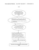
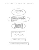
[0009] FIG. 1 is a flowchart depicting the breakup of the method for determining the heat boundary value conditions of a myocardial sample within the left ventricle of a heart according to the present invention.
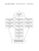
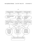
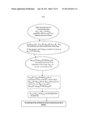
[0010] FIG. 2 is a flowchart depicting the cursory process flow for obtaining radial, longitudinal, and circumferential components of the magnitude of heat generated or lost at apical, mid, and basal anterior which, in turn, are transferred to the neighboring red blood cells.
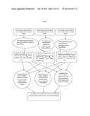
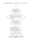
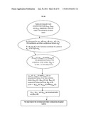
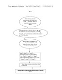
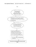
[0011] FIG. 3 is a flowchart depicting the method for obtaining radial, longitudinal, and circumferential components of the magnitude of heat generated or lost at apical anterior through parameterized elements.
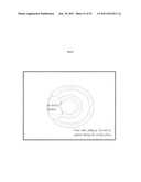
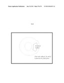
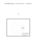
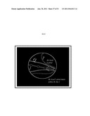
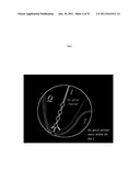
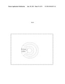
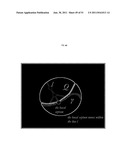
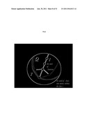
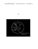
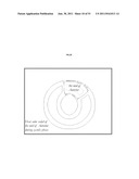
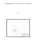
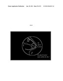
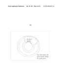
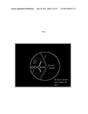
[0012] FIG. 4 is a rendering of the apical anterior moving within its corresponding parameterized forms of lines.
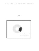
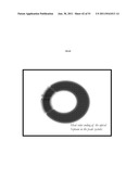
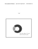
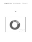
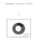
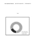
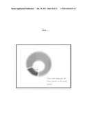
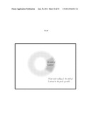
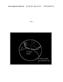
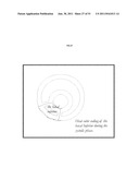
[0013] FIG. 5 is a rendering of the color-coded representation of the distribution of heat of the apical anterior at peak systolic using Mathlab software.
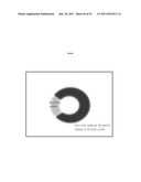
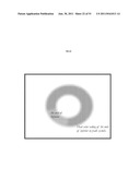
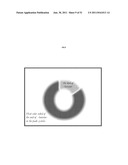
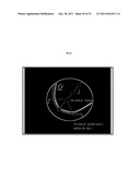
[0014] FIG. 6 is a rendering of the color-coded representation of the distribution of heat of the apical anterior during the entire systolic phase using Mathlab software.
[0015] FIG. 7 is a flowchart depicting the method for obtaining radial, longitudinal, and circumferential components of the magnitude of heat generated or lost at mid anterior through parameterized elements.
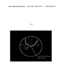
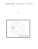
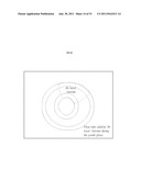
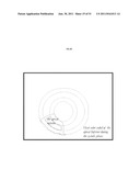
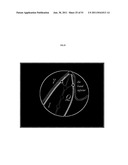
[0016] FIG. 8 is a rendering of the mid anterior moving within its corresponding parameterized forms of lines.
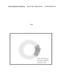
[0017] FIG. 9 is a rendering of the color-coded representation of the distribution of heat of the mid anterior at peak systolic using Mathlab software.
[0018] FIG. 10 is a rendering of the color-coded representation of the distribution of heat of the mid anterior during the entire systolic phase using Mathlab software.
[0019] FIG. 11 is a flowchart depicting the method for obtaining radial, longitudinal, and circumferential components of the magnitude of heat generated or lost at basal anterior through parameterized elements.
[0020] FIG. 12 is a rendering of the basal anterior moving within its corresponding parameterized forms of lines.
[0021] FIG. 13 is a rendering of the color-coded representation of the distribution of heat of the basal anterior at peak systolic using Mathlab software.
[0022] FIG. 14 is a rendering of the color-coded representation of the distribution of heat of the basal anterior during the entire systolic phase using Mathlab software.
[0023] FIG. 15 is a flowchart depicting the cursory process flow for obtaining radial, longitudinal, and circumferential components of the magnitude of heat generated or lost at apical, mid, and basal inferior which, in turn, are transferred to the neighboring red blood cells.
[0024] FIG. 16 is a flowchart depicting the method for obtaining radial, longitudinal, and circumferential components of the magnitude of heat generated or lost at apical inferior through parameterized elements.
[0025] FIG. 17 is a rendering of the apical inferior moving within its corresponding parameterized forms of lines.
[0026] FIG. 18 is a rendering of the color-coded representation of the distribution of heat of the apical inferior at peak systolic using Mathlab software.
[0027] FIG. 19 is a rendering of the color-coded representation of the distribution of heat of the apical inferior during the entire systolic phase using Mathlab software.
[0028] FIG. 20 is a flowchart depicting the method for obtaining radial, longitudinal, and circumferential components of the magnitude of heat generated or lost at mid inferior through parameterized elements.
[0029] FIG. 21 is a rendering of the mid inferior moving within its corresponding parameterized forms of lines.
[0030] FIG. 22 is a rendering of the color-coded representation of the distribution of heat of the mid inferior at peak systolic using Mathlab software.
[0031] FIG. 23 is a rendering of the color-coded representation of the distribution of heat of the mid inferior during the entire systolic phase using Mathlab software.
[0032] FIG. 24 is a flowchart depicting the method for obtaining radial, longitudinal, and circumferential components of the magnitude of heat generated or lost at basal inferior through parameterized elements.
[0033] FIG. 25 is a rendering of the basal inferior moving within its corresponding parameterized forms of lines.
[0034] FIG. 26 is a rendering of the color-coded representation of the distribution of heat of the basal inferior at peak systolic using Mathlab software.
[0035] FIG. 27 is a rendering of the color-coded representation of the distribution of heat of the basal inferior during the entire systolic phase using Mathlab software.
[0036] FIG. 28 is a flowchart depicting the method for obtaining radial, longitudinal, and circumferential components of the magnitude of heat generated or lost at apical lateral through parameterized elements.
[0037] FIG. 29 is a rendering of the apical lateral moving within its corresponding parameterized forms of lines.
[0038] FIG. 30 is a rendering of the color-coded representation of the distribution of heat of the apical lateral at peak systolic using Mathlab software.
[0039] FIG. 31 is a rendering of the color-coded representation of the distribution of heat of the apical lateral during the entire systolic phase using Mathlab software.
[0040] FIG. 32 is a flowchart depicting the method for obtaining radial, longitudinal, and circumferential components of the magnitude of heat generated or lost at mid lateral through parameterized elements.
[0041] FIG. 33 is a rendering of the mid lateral moving within its corresponding parameterized forms of lines.
[0042] FIG. 34 is a rendering of the color-coded representation of the distribution of heat of the mid lateral at peak systolic using Mathlab software.
[0043] FIG. 35 is a rendering of the color-coded representation of the distribution of heat of the mid lateral during the entire systolic phase using Mathlab software.
[0044] FIG. 36 is a flowchart depicting the method for obtaining radial, longitudinal, and circumferential components of the magnitude of heat generated or lost at basal lateral through parameterized elements.
[0045] FIG. 37 is a rendering of the basal lateral moving within its corresponding parameterized forms of lines.
[0046] FIG. 38 is a rendering of the color-coded representation of the distribution of heat of the basal lateral at peak systolic using Mathlab software.
[0047] FIG. 39 is a rendering of the color-coded representation of the distribution of heat of the basal lateral during the entire systolic phase using Mathlab software.
[0048] FIG. 40 is a flowchart depicting the method for obtaining radial, longitudinal, and circumferential components of the magnitude of heat generated or lost at apical septum through parameterized elements.
[0049] FIG. 41 is a rendering of the apical septum moving within its corresponding parameterized forms of lines.
[0050] FIG. 42 is a rendering of the color-coded representation of the distribution of heat of the apical septum at peak systolic using Mathlab software.
[0051] FIG. 43 is a rendering of the color-coded representation of the distribution of heat of the apical septum during the entire systolic phase using Mathlab software.
[0052] FIG. 44 is a flowchart depicting the method for obtaining radial, longitudinal, and circumferential components of the magnitude of heat generated or lost at mid septum through parameterized elements.
[0053] FIG. 45 is a rendering of the mid septum moving within its corresponding parameterized forms of lines.
[0054] FIG. 46 is a rendering of the color-coded representation of the distribution of heat of the mid septum at peak systolic using Mathlab software.
[0055] FIG. 47 is a rendering of the color-coded representation of the distribution of heat of the mid septum during the entire systolic phase using Mathlab software.
[0056] FIG. 48 is a flowchart depicting the method for obtaining radial, longitudinal, and circumferential components of the magnitude of heat generated or lost at basal septum through parameterized elements.
[0057] FIG. 49 is a rendering of the basal septum moving within its corresponding parameterized forms of lines.
[0058] FIG. 50 is a rendering of the color-coded representation of the distribution of heat of the basal septum at peak systolic using Mathlab software.
[0059] FIG. 51 is a rendering of the color-coded representation of the distribution of heat of the basal septum during the entire systolic phase using Mathlab software.
DETAILED DESCRIPTION
[0060] In the following detailed description, a reference is made to the accompanying drawings that form a part hereof, and in which the specific embodiments that may be practiced is shown by way of illustration. These embodiments are described in sufficient detail to enable those skilled in the art to practice the embodiments and it is to be understood that the logical, mechanical and other changes may be made without departing from the scope of the embodiments. The following detailed description is therefore not to be taken in a limiting sense.
[0061] The present invention describes a computer-implemented method for determining the heat boundary value conditions of red blood cells in the neighborhood of a myocardium pertaining to the left ventricle of a heart. The heat boundary value conditions are determined at apical, mid, and basal positions of the myocardium in that order wherein, the apical and basal positions are the positions at which the systolic phase of the heart starts and ends respectively. The mid position, as the term suggests, is centered between the apical and basal positions. The heat boundary value conditions comprise radial, longitudinal, and circumferential components of the magnitude of heat transferred from the myocardium to the neighboring red blood cells. The method of the present invention is a part of the comprehensive study of myocardial behavior relative to heat.
[0062] Referring to FIG. 1, the myocardium is divided into a plurality of myocardial samples wherein, each comprises a four myocardial surfaces viz., anterior, inferior, lateral, and septum.
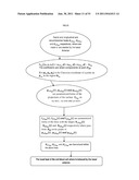
[0063] Apical Anterior: Referring to FIGS. 2 and 3, the anterior surface of a myocardial sample at the apical position (hereinafter "apical anterior") and the neighborhood thereof are represented by PaA and OaA respectively. The surface of the apical anterior PaA is, in turn, quadratically represented by the following equation:
FPaA(y1,y2,y3)=εrr,PaAy1- 2+εll,PaAy22+εcc,PaAy.s- ub.32-DPaA
wherein, FPaA is the quadratic surface of the apical anterior PaA, (y1y2y3) represent the Cartesian coordinates of a point on a myofiber curve passing from the apical anterior PaA in the neighborhood OaA, the co-efficients εrr,PaA, εrr,PaA, and εrr,PaA are the strain components at the apical anterior PaA, and DPaA is the displacement of the apical anterior PaA from the apical position. The myofiber curve is represented by γPaA, which, in turn, is quadratically represented by QPaA.
[0064] Let the parameterized forms of projections of the apical anterior surface FPaA on x-y, x-z, and y-z axes are represented by φ1,PaA (t), φ2,PaA (t), and φ3,PaA (t) respectively. Based on the parameterized forms of projections, parameterized forms of lines are formulized within which the apical anterior surface FPaA moves as shown in FIG. 4. The parameterized forms of lines along x-y, x-z, and y-z axes are represented by the following equations:
l1,PaA(t):={(x,y);(x,y)T1,PaA(t)=0};
l2,PaA(t):={(x,z);(x,z)T2,PaA(t)=0};
l3,PaA(t):={(y,z);(y,z)T3,PaA(t)=0};
wherein, l1,PaA (t), l2,PaA (t), and l3,PaA (t) represent the parameterized forms of lines along x-y, x-z, and y-z axes respectively, and t represents the time taken for the apical anterior to reach its position with respect to the apical position.
[0065] Once the parameterized forms of lines are l1,PaA (t), l2,PaA (t), and l3,PaA (t) are formulized, the radial, longitudinal, and circumferential components of the magnitude of heat generated or lost at the apical anterior are obtained by the following formulae:
Hr,PaA(t):=a1,PaA(t)μVolume(t)/εrr,P- aA×DPaA(t);
Hl,PaA(t):=a2,PaA(t)μVolume(t)/εll,P- aA×DPaA(t);
Hc,PaA(t):=a3,PaA(t)μVolume(t)/εcc,P- aA×DPaA(t);
wherein, Hr,PaA (t), Hl,PaA(t), and Hc,PaA (t) represent the radial, longitudinal, and circumferential components of the magnitude of heat generated or lost at the apical anterior respectively, a1,PaA (t), a2,PaA (t), and a3,PaA (t) represent the gravity of the apical anterior within l1,PaA (t), l2,PaA (t), and l3,PaA (t) respectively, and μ and Volume(t) represent the density and volume of the corresponding myocardial sample respectively.
[0066] If (x1, x2, x3, t) are the coordinates of a red blood cell in the neighborhood OaA, then δ(x1, x2, x3, t)=δ'(x1,t)δ'(x2,t)δ'(x3,t) wherein, δ' represents Dirac function. The radial, longitudinal, and circumferential components of the magnitude of heat transferred from the apical anterior to the red blood cells in the neighborhood OaA are determined by the following formulae:
Hr,PaARBC(t)=∫C1PaAHr,P.sub- .aA(t)δ(x1,x2,x3,t)dt;
Hl,PaARBC(t)=∫C2PaAHl,P.sub- .aA(t)δ(x1,x2,x3,t)dt;
Hc,PaARBC(t)=∫C3PaAHc,P.sub- .aA(t)δ(x1,x2,x3,t)dt;
wherein, C1,PaA, C2,PaA, and C3,PaA are the graphs of φ1,PaA (t), φ2,PaA (t), and φ3,PaA (t) respectively.
[0067] Based on the values obtained from the above formulae, the color-coded representation of the distribution of heat of the apical anterior at peak systolic and during the entire systolic phase are obtained as shown respectively in FIGS. 5 and 6.
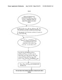
[0068] Mid Anterior: Referring to FIGS. 2 and 7, the anterior surface of a myocardial sample at the mid position (hereinafter "mid anterior") and the neighborhood thereof are represented by PmA and OmA respectively. The surface of the mid anterior PmA is, in turn, quadratically represented by the following equation:
FPmA(y1,y2,y3)=εrr,PmAy1- 2+εll,PmAy22+εcc,PmAy.s- ub.32-DPmA
wherein, FPmA is the quadratic surface of the mid anterior PmA, (y1,y2,y3,) represent the Cartesian coordinates of a point on a myofiber curve passing from the mid anterior PmA in the neighborhood OmA, the co-efficients εrr,PmA,εrr,PmA, and εrr,PmA are the strain components at the mid anterior PmA, and DPmA is the displacement of the mid anterior PmA from the mid position. The myofiber curve is represented by γpmA, which, in turn, is quadratically represented by QPmA.
[0069] Let the parameterized forms of projections of the mid anterior surface FPmA on x-y, x-z, and y-z axes are represented by φ1,PmA (t), φ2,PmA (t), and φ3,PmA (t) respectively. Based on the parameterized forms of projections, parameterized forms of lines are formulized within which the mid anterior surface FPmA moves as shown in FIG. 8. The parameterized forms of lines along x-y, x-z, and y-z axes are represented by the following equations:
l1,PmA(t):={(x,y);(x,y)T1,PmA(t)=0};
l2,PmA(t):={(x,z);(x,z)T2,PmA(t)=0};
l3,PmA(t):={(y,z);(y,z)T3,PmA(t)=0};
wherein, l1,PmA(t), l2,PmA(t), and l3,PmA(t) represent the parameterized forms of lines along x-y, x-z, and y-z axes respectively, and t represents the time taken for the mid anterior to reach its position from the apical position.
[0070] Once the parameterized forms of lines l1,PmA(t), l2,PmA(t), and l3,PmA(t) are formulized, the radial, longitudinal, and circumferential components of the magnitude of heat generated or lost at the mid anterior are obtained by the following formulae:
Hr,PmA(t):=a1,PmA(t)μVolume(t)/εrr,P- mA×DPmA(t);
Hl,PmA(t):=a2,PmA(t)μVolume(t)/εll,P- mA×DPmA(t);
Hc,PmA(t):=a3,PmA(t)μVolume(t)/εcc,P- mA×DPmA(t);
wherein, Hr,PmA(t), Hl,PmA(t), and Hc,PmA(t) represent the radial, longitudinal, and circumferential components of the magnitude of heat generated or lost at the mid anterior respectively, a1,PmA(t), a2,PmA(t), and a3,PmA(t) represent the gravity of the mid anterior within l1,PmA(t), l2,PmA(t), and l3,PmA(t) respectively, and μ and Volume(t) represent the density and volume of the corresponding myocardial sample respectively.
[0071] If (x1, x2, x3, t) are the coordinates of a red blood cell in the neighborhood OmA, then δ(x1, x2,x3, t)=δ'(x1,t,)δ'(x2,t)δ'(x3,t) wherein, δ' represents Dirac function. The radial, longitudinal, and circumferential components of the magnitude of heat transferred from the mid anterior to the red blood cells in the neighborhood OmA are determined by the following formulae:
Hr,PmARBC(t)=∫C1.sub.,PmAHr,P.su- b.mA(t)δ(x1,x2,x3,t)dt;
Hl,PmARBC(t)=∫C2.sub.,PmAHl,P.su- b.mA(t)δ(x1,x2,x3,t)dt;
Hc,PmARBC(t)=∫C3.sub.,PmAHc,P.su- b.mA(t)δ(x1,x2,x3,t)dt;
wherein, C l,PmA, C2,PmA, and C3,PmA are the graphs of φ1,PmA(t), φ2,PmA(t), and φ3,PmA(t) respectively.
[0072] Based on the values obtained from the above formulae, the color-coded representation of the distribution of heat of the mid anterior at peak systolic and during the entire systolic phase are obtained as shown respectively in FIGS. 9 and 10.
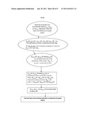
[0073] Basal Anterior: Referring to FIGS. 2 and 11, the anterior surface of a myocardial sample at the basal position (hereinafter "basal anterior") and the neighborhood thereof are represented by PbA and ObA respectively. The surface of the basal anterior PbA is, in turn, quadratically represented by the following equation:
FPbA(y1,y2,y3)=εrr,PbAy1- 2+εll,PbAy22+εcc,PbAy.s- ub.32-DPbA
wherein, FPbA is the quadratic surface of the basal anterior PbA, (y1y2,y3) represent the Cartesian coordinates of a point on a myofiber curve passing from the basal anterior PbA in the neighborhood ObA, the co-efficients εrr,PbA,εrr,PbA, and εrr,PbA are the strain components at the basal anterior PbA, and DPbA is the displacement of the basal anterior PbA from the mid position. The myofiber curve is represented by γPbA , which, in turn, is quadratically represented by QPbA.
[0074] Let the parameterized forms of projections of the basal anterior surface FPbA on x-y, x-z, and y-z axes are represented by φ1,PbA(t), φ2,PbA(t), and φ3,PbA(t) respectively. Based on the parameterized forms of projections, parameterized forms of lines are formulized within which the basal anterior surface FPbA moves as shown in FIG. 12. The parameterized forms of lines along x-y, x-z, and y-z axes are represented by the following equations:
l1,PbA(t):={(x,y);(x,y)T1,PbA(t)=0};
l2,PbA(t):={(x,z);(x,z)T2,PbA(t)=0};
l3,PbA(t):={(y,z);(y,z)T3,PbA(t)=0};
wherein, l1,PbA(t), l2,PbA(t), and l3,PbA(t) represent the parameterized forms of lines along x-y, x-z, and y-z axes respectively, and t represents the time taken for the basal anterior to reach its position from the apical position.
[0075] Once the parameterized forms of lines l1,PbA(t), l2,PbA(t), and l3,PbA(t) are formulized, the radial, longitudinal, and circumferential components of the magnitude of heat generated or lost at the basal anterior are obtained by the following formulae:
Hr,PbA(t):=a1,PbA(t)μVolume(t)/εrr,P- bA×DPbA(t);
Hl,PbA(t):=a2,PbA(t)μVolume(t)/εll,P- bA×DPbA(t);
Hc,PbA(t):=a3,PbA(t)μVolume(t)/εcc,P- bA×DPbA(t);
wherein, Hr,PbA(t), Hl,PbA(t), and Hc,PbA(t) represent the radial, longitudinal, and circumferential components of the magnitude of heat generated or lost at the basal anterior respectively, a1,PbA(t), a2,PbA(t), and a3,PbA(t) represent the gravity of the basal anterior within l1,PbA(t), l2,PbA(t), and l3,Pb(t) respectively, and μ and Volume(t) represent the density and volume of the corresponding myocardial sample respectively.
[0076] If (x1, x2, x3, t) are the coordinates of a red blood cell in the neighborhood OmA, then δ(x1, x2, x3, t)=δ'(x1,t)δ'(x3,t) wherein, δ' represents Dirac function. The radial, longitudinal, and circumferential components of the magnitude of heat transferred from the basal anterior and the red blood cells in the neighborhood ObA are determined by the following formulae:
Hr,PbARBC(t)=∫C1.sub.,PbAHr,P.su- b.bA(t)δ(x1,x2,x3,t)dt;
Hl,PbARBC(t)=∫C2.sub.,PbAHl,P.su- b.bA(t)δ(x1,x2,x3,t)dt;
Hc,PbARBC(t)=∫C3.sub.,PbAHc,P.su- b.bA(t)δ(x1,x2,x3,t)dt;
wherein, Cl,PbA, C2,PbA, and C3,PbA are the graphs of φ1,PbA(t), φ2,PbA(t), and φ3,PbA(t) respectively.
[0077] Based on the values obtained from the above formulae, the color-coded representation of the distribution of heat of the basal anterior at peak systolic and during the entire systolic phase are obtained as shown respectively in FIGS. 13 and 14.
[0078] Apical Inferior: Referring to FIGS. 15 and 16, the inferior surface of a myocardial sample at the apical position (hereinafter "apical inferior") and the neighborhood thereof are represented by Pal and Oal respectively. The surface of the apical inferior Pal is, in turn, quadratically represented by the following equation:
FPal(y1,y2,y3)=εrr,Paly1- 2+εll,Paly22+εcc,Paly.s- ub.32-DPal
wherein, FPal is the quadratic surface of the apical inferior Pal, (y1,y2,y3) represent the Cartesian coordinates of a point on a myofiber curve passing from the apical inferior Pal in the neighborhood Oal, the co-efficients εrr,Pal,εrr,Pal, and εrr,Pal are the strain components at the apical inferior Pal, and DPal is the displacement of the apical inferior Pal from the apical position. The myofiber curve is represented by γPal, which, in turn, is quadratically represented by QPal.
[0079] Let the parameterized forms of projections of the apical inferior surface FPal on x-y, x-z, and y-z axes are represented by φ1,Pal(t), φ2,Pal(t), and φ3,Pal(t) respectively. Based on the parameterized forms of projections, parameterized forms of lines are formulized within which the apical inferior surface FPal moves as shown in FIG. 17. The parameterized forms of lines along x-y, x-z, and y-z axes are represented by the following equations:
l1,Pal(t):={(x,y);(x,y)T1,Pal(t)=0};
l2,Pal(t):={(x,z);(x,z)T2,Pal(t)=0};
l3,Pal(t):={(y,z);(y,z)T3,Pal(t)=0};
wherein, l1,Pal(t), l2,Pal(t), and l3,Pal(t) represent the parameterized forms of lines along x-y, x-z, and y-z axes respectively, and t represents the time taken for the apical inferior to reach its position from the apical position.
[0080] Once the parameterized forms of lines l1,Pal(t), l2,Pal(t), and l3,Pal(t) are formulized, the radial, longitudinal, and circumferential components of the magnitude of heat generated or lost at the apical inferior are obtained by the following formulae:
Hr,Pal(t):=a1,Pal(t)μVolume(t)/εrr,P- al×DPal(t);
Hl,Pal(t):=a2,Pal(t)μVolume(t)/εll,P- al×DPal(t);
Hc,Pal(t):=a3,Pal(t)μVolume(t)/εcc,P- al×DPal(t);
wherein, Hr,Pal(t), Hl,Pal(t), and Hc,Pal(t) represent the radial, longitudinal, and circumferential components of the magnitude of heat generated or lost at the apical inferior respectively, a1,Pal(t), a2,Pal(t), and a3,Pal(t) represent the gravity of the apical inferior within 1l1,Pal(t), l2,Pal(t), and l3,Pal(t) respectively, and μ and Volume(t) represent the density and volume of the corresponding myocardial sample respectively.
[0081] If (x1, x2, x3, t) are the coordinates of a red blood cell in the neighborhood Oal, then δ(x1, x2, x3, t)=δ'(x1,t) (x2,t)δ'(x3,t) wherein, δ' represents Dirac function. The radial, longitudinal, and circumferential components of the magnitude of heat transferred from the apical inferior to the red blood cells in the neighborhood Oal are determined by the following formulae:
Hr,PalRBC(t)=∫C1.sub.,PalHr,P.su- b.al(t)δ(x1,x2,x3,t)dt;
Hl,PalRBC(t)=∫C2.sub.,PalHl,P.su- b.al(t)δ(x1,x2,x3,t)dt;
Hc,PalRBC(t)=∫C3.sub.,PalHc,P.su- b.al(t)δ(x1,x2,x3,t)dt;
[0082] wherein, C1,Pal, C2,Pal, and C3,Pal are the graphs of φ1,Pal(t), φ2,Pal(t), and φ3,Pal(t) respectively.
[0083] Based on the values obtained from the above formulae, the color-coded representation of the distribution of heat of the apical inferior at peak systolic and during the entire systolic phase are obtained as shown respectively in FIGS. 18 and 19.
[0084] Mid Inferior: Referring to FIGS. 15 and 20, the inferior surface of a myocardial sample at the mid position (hereinafter "mid inferior") and the neighborhood thereof are represented by Pml, and Oml respectively. The surface of the mid inferior Pml is, in turn, quadratically represented by the following equation:
FPml(y1,y2,y3)=εrr,Pmly1- 2+εll,Pmly22+εcc,Pmly.s- ub.32-DPml
wherein, FPml is the quadratic surface of the mid inferior Pml, (y1,y2,y3) represent the Cartesian coordinates of a point on a myofiber curve passing from the mid inferior Pml in the neighborhood Oml, the co-efficients εrr,Pml, εrr,Pml, and εrr,Pml are the strain components at the mid inferior Pml, and DPml is the displacement of the mid inferior Pml from the apical position. The myofiber curve is represented by γPml, which, in turn, is quadratically represented by φPml.
[0085] Let the parameterized forms of projections of the mid inferior surface FPml on x-y, x-z, and y-z axes are represented by φ1,Pml(t), φ2,Pml(t), and φ3,Pml(t) respectively. Based on the parameterized forms of projections, parameterized forms of lines are formulized within which the mid inferior surface FPml moves as shown in FIG. 21. The parameterized forms of lines along x-y, x-z, and y-z axes are represented by the following equations:
l1,Pml(t):={(x,y);(x,y)T1,Pml(t)=0};
l2,Pml(t):={(x,z);(x,z)T2,Pml(t)=0};
l3,Pml(t):={(y,z);(y,z)T3,Pml(t)=0};
[0086] wherein, l1,Pml(t), l2,Pml(t), and l3,Pml(t) represent the parameterized forms of lines along x-y, x-z, and y-z axes respectively, and I represents the time taken for the mid inferior to reach its position from the apical position.
[0087] Once the parameterized forms of lines l1,Pml(t), l2,Pml(t), and l3,Pml(t) are formulized, the radial, longitudinal, and circumferential components of the magnitude of heat generated or lost at the mid inferior are obtained by the following formulae:
Hr,Pml(t):=a1,Pml(t)μVolume(t)/εrr,P- ml×DPml(t);
Hl,Pml(t):=a2,Pml(t)μVolume(t)/εll,P- ml×DPml(t);
Hc,Pml(t):=a3,Pml(t)μVolume(t)/εcc,P- ml×DPml(t);
wherein, Hr,Pml(t), Hl,Pml(t) , and Hc,Pml(t) represent the radial, longitudinal, and circumferential components of the magnitude of heat generated or lost at the mid inferior respectively, a1,Pml(t), a2,Pml(t), and a3,Pml(t) represent the gravity of the mid inferior within l1,Pml(t), l2,Pml(t), and l3,Pml(t) respectively, and μ and Volume(t) represent the density and volume of the corresponding myocardial sample respectively.
[0088] If (x1, x2, x3, t) are the coordinates of a red blood cell in the neighborhood Oml, then δ(x1, x2,x3, t)=δ'(x1,t)δ'(x2,t)δ'(x3,t) wherein, δ' represents Dirac function. The radial, longitudinal, and circumferential components of the magnitude of heat transferred from the mid inferior to the red blood cells in the neighborhood Oml are determined by the following formulae:
Hr,PmlRBC(t)=∫C1.sub.,PmlHr,P.su- b.ml(t)δ(x1,x2,x3,t)dt;
Hl,PmlRBC(t)=∫C2.sub.,PmlHl,P.su- b.ml(t)δ(x1,x2,x3,t)dt;
Hc,PmlRBC(t)=∫C3.sub.,PmlHc,P.su- b.ml(t)δ(x1,x2,x3,t)dt;
[0089] wherein, C1,Pml, C2,Pml, and C3,Pml are the graphs of φ1,Pml(t), φ2,Pml(t), and φ3,Pml(t) respectively.
[0090] Based on the values obtained from the above formulae, the color-coded representation of the distribution of heat of the mid inferior at peak systolic and during the entire systolic phase are obtained as shown respectively in FIGS. 22 and 23.
[0091] Basal Inferior: Referring to FIGS. 15 and 24, the inferior surface of a myocardial sample at the basal position (hereinafter "basal inferior") and the neighborhood thereof are represented by Pbl and Obl respectively. The surface of the basal inferior Pbl is, in turn, quadratically represented by the following equation:
FPbl(y1,y2,y3)=εrr,Pbly1- 2+εll,Pbly22+εcc,Pbly.s- ub.32-DPbl
wherein, FPbl is the quadratic surface of the basal inferior Pbl, (y1,y2,y3) represent the Cartesian coordinates of a point on a myofiber curve passing from the basal inferior Pbl in the neighborhood Obl, the co-efficients εrr,Pbl,εrr,Pbl, and εrr,Pbl are the strain components at the basal inferior Pbl, and DPbl is the displacement of the mid inferior Pbl from the apical position. The myofiber curve is represented by γhd Pbl, which, in turn, is quadratically represented by QPbl.
[0092] Let the parameterized forms of projections of the basal inferior surface FPbl on x-y, x-z, and y-z axes are represented by φ1,Pbl(t), φ2,Pbl(t), and φ3,Pbl(t) respectively. Based on the parameterized forms of projections, parameterized forms of lines are formulized within which the basal inferior surface FPbl moves as shown in FIG. 25. The parameterized forms of lines along x-y, x-z, and y-z axes are represented by the following equations:
l1,Pbl(t):={(x,y);(x,y)T1,Pbl(t)=0};
l2,Pbl(t):={(x,z);(x,z)T2,Pbl(t)=0};
l3,Pbl(t):={(y,z);(y,z)T3,Pbl(t)=0};
[0093] wherein, l1,Pbl(t), l2,Pbl(t), and l3,Pbl(t) represent the parameterized forms of lines along x-y, x-z, and y-z axes respectively, and t represents the time taken for the mid inferior to reach its position from the apical position.
[0094] Once the parameterized forms of lines l1,Pbl(t), l2,Pb1(t), and l3,Pbl(t) are formulized, the radial, longitudinal, and circumferential components of the magnitude of heat generated or lost at the basal inferior are obtained by the following formulae:
Hr,Pbl(t):=a1,Pbl(t)μVolume(t)/εrr,P- l×DPbl(t);
Hl,Pbl(t):=a2,Pbl(t)μVolume(t)/εll,P- bl×DPbl(t);
Hc,Pbl(t):=a3,Pbl(t)μVolume(t)/εcc,P- bl×DPbl(t);
wherein, Hr,Pbl(t), Hl,Pbl(t), and Hc,Pbl(t) represent the radial, longitudinal, and circumferential components of the magnitude of heat generated or lost at the basal inferior respectively, a1,Pbl(t), a2,Pbl(t), and a3,Pbl(t) represent the gravity of the basal inferior within l1,Pbl(t), l2,Pbl(t), and l3,Pbl(t) respectively, and μ and Volume(t) represent the density and volume of the corresponding myocardial sample respectively.
[0095] If (x1, x2, x3, t) are the coordinates of a red blood cell in the neighborhood Obl, then δ(x1,x2,x3,t)=δ'(x1,t)δ'(x2,t)- δ'(x3,t) wherein, δ' represents Dirac function. The radial, longitudinal, and circumferential components of the magnitude of heat transferred from the basal inferior to the red blood cells in the neighborhood Obl are determined by the following formulae:
Hr,PblRBC(t)=∫C1.sub.,PblHr,P.su- b.bl(t)δ(x1,x2,x3,t)dt;
Hl,PblRBC(t)=∫C2.sub.,PblHl,P.su- b.bl(t)δ(x1,x2,x3,t)dt;
Hc,PblRBC(t)=∫C3.sub.,PblHc,P.su- b.bl(t)δ(x1,x2,x3,t)dt;
wherein, C1,Pbl, C2,Pbl, and C3,Pbl are the graphs of φ1,Pbl(t), φ2,Pbl(t), and φ3,Pbl(t) respectively.
[0096] Based on the values obtained from the above formulae, the color-coded representation of the distribution of heat of the basal inferior at peak systolic and during the entire systolic phase are obtained as shown respectively in FIGS. 26 and 27.
[0097] Apical Lateral: Referring to FIG. 28, the lateral surface of a myocardial sample at the apical position (hereinafter "apical lateral") and the neighborhood thereof are represented by PaL and OaL respectively. The surface of the lateral inferior PaL is, in turn, quadratically represented by the following equation:
FPaL(y1,y2,y3)=εrr,PaLy1- 2+εll,PaLy22+εcc,PaLy.s- ub.32-DPaL
wherein, FPaL is the quadratic surface of the apical lateral PaL, (y1,y2,y3) represent the Cartesian coordinates of a point on a myofiber curve passing from the apical lateral PaL in the neighborhood OaL, the co-efficients εrr,PaL,εrr,PaL and εrr,PaL are the strain components at the apical lateral PaL, and DPaL is the displacement of the apical lateral PaL from the apical position. The myofiber curve is represented by γPaL, which, in turn, is quadratically represented by QPaL.
[0098] Let the parameterized forms of projections of the apical lateral surface FPaL on x-y, x-z, and y-z axes are represented by φ1,PaL(t), φ2,PaL(t), and φ3,PaL(t) respectively. Based on the parameterized forms of projections, parameterized forms of lines are formulized within which the apical lateral surface FPaL moves as shown in FIG. 29. The parameterized forms of lines along x-y, x-z, and y-z axes are represented by the following equations:
l1,PaL(t):={(x,y);(x,y)T1,PaL(t)=0};
l2,PaL(t):={(x,z);(x,z)T2,PaL(t)=0};
l3,PaL(t):={(y,z);(y,z)T3,PaL(t)=0};
[0099] wherein, l1,PaL(t), l2,PaL(t), and l3,PaL(t) represent the parameterized forms of lines along x-y, x-z, and y-z axes respectively, and t represents the time taken for the apical lateral to reach its position from the apical position.
[0100] Once the parameterized forms of lines l1,PaL(t), l2,PaL(t), and l3,PaL(t) are formulized, the radial, longitudinal, and circumferential components of the magnitude of heat generated or lost at the apical lateral are obtained by the following formulae:
Hr,PaL(t):=a1,PaL(t)μVolume(t)/εrr,P- aL×DPaL(t);
Hl,PaL(t):=a2,PaL(t)μVolume(t)/εll,P- aL×DPaL(t);
Hc,PaL(t):=a3,PaL(t)μVolume(t)/εcc,P- aL×DPaL(t);
wherein, Hr,PaL(t), Hl,PaL(t), and Hc,PaL (t) represent the radial, longitudinal, and circumferential components of the magnitude of heat generated or lost at the apical lateral respectively, a1,PpaL(t), a2,PaL(t), and a3,PaL(t) represent the gravity of the apical lateral within l1,PaL(t), l2,PaL(t), and l3,PaL(t) respectively, and μ and Volume(t) represent the density and volume of the corresponding myocardial sample respectively.
[0101] If (x1, x2, x3, t) are the coordinates of a red blood cell in the neighborhood OaL, then δ(x1,x2,x3,t)=δ'(x1,t)δ'(x2,t)- δ'(x3,t) wherein, δ' represents Dirac function. The radial, longitudinal, and circumferential components of the magnitude of heat transferred from the apical lateral to the red blood cells in the neighborhood OaL are determined by the following formulae:
Hr,PaLRBC(t)=∫C1.sub.,PaLHr,P.su- b.aL(t)δ(x1,x2,x3,t)dt;
Hl,PaLRBC(t)=∫C2.sub.,PaLHl,P.su- b.aL(t)δ(x1,x2,x3,t)dt;
Hc,PaLRBC(t)=∫C3.sub.,PaLHc,P.su- b.aL(t)δ(x1,x2,x3,t)dt;
wherein, C1,PaL, C2,PaL, and C3,PaL are the graphs of φ1,PaL(t), φ2,PaL(t), and φ3,PaL(t) respectively.
[0102] Based on the values obtained from the above formulae, the color-coded representation of the distribution of heat of the apical lateral at peak systolic and during the entire systolic phase are obtained as shown respectively in FIGS. 30 and 31.
[0103] Mid Lateral: Referring to FIG. 32, the lateral surface of a myocardial sample at the mid position (hereinafter "mid lateral") and the neighborhood thereof are represented by PmL and OmL respectively. The surface of the mid lateral PmL is, in turn, quadratically represented by the following equation:
FPmL(y1,y2,y3)=εrr,PmLy1- 2+εll,PmLy22+εcc,PmLy.s- ub.32-DPmL
wherein, FPmL is the quadratic surface of the mid lateral PmL, (y1,y2,y3) represent the Cartesian coordinates of a point on a myofiber curve passing from the mid lateral PmL in the neighborhood OmL, the co-efficients εrr,PmL,εrr,PmL, and εrr,PmL are the strain components at the mid lateral PmL, and DPmL is the displacement of the mid lateral PmL from the apical position. The myofiber curve is represented by γPmL, which, in turn, is quadratically represented by QPmL.
[0104] Let the parameterized forms of projections of the mid lateral surface FPmL on x-y, x-z, and y-z axes are represented by φ1,PmL(t), φ2,PmL(t), and φ3,PmL(t) respectively. Based on the parameterized forms of projections, parameterized forms of lines are formulized within which the mid lateral surface FPmL moves as shown in FIG. 33. The parameterized forms of lines along x-y, x-z, and y-z axes are represented by the following equations:
l1,PmL(t):={(x,y);(x,y)T1,PmL(t)=0};
l2,PmL(t):={(x,z);(x,z)T2,PmL(t)=0};
l3,PmL(t):={(y,z);(y,z)T3,PmL(t)=0};
wherein, l1,PmL(t), l2,PmL(t), and l3,PmL(t) represent the parameterized forms of lines along x-y, x-z, and y-z axes respectively, and t represents the time taken for the mid lateral to reach its position from the apical position.
[0105] Once the parameterized forms of lines l1,PmL(t), l2,PmL(t), and l3,PmL(t) are formulized, the radial, longitudinal, and circumferential components of the magnitude of heat generated or lost at the mid lateral are obtained by the following formulae:
Hr,PmL(t):=a1,PmL(t)μVolume(t)/εrr,P- mL×DPmL(t);
Hl,PmL(t):=a2,PmL(t)μVolume(t)/εll,P- mL×DPmL(t);
Hc,PmL(t):=a3,PmL(t)μVolume(t)/εcc,P- mL×DPmL(t);
wherein, Hr,PmL(t), Hl,PmL(t), and Hc,PmL(t) represent the radial, longitudinal, and circumferential components of the magnitude of heat generated or lost at the mid lateral respectively, a1,PmL(t), a2,PmL(t), and a3,PmL(t) represent the gravity of the mid lateral within l1,PmL(t), l2,PmL(t) , and l3,PmL(t) respectively, and μ and Volume(t) represent the density and volume of the corresponding myocardial sample respectively.
[0106] If (x1, x2, x3, t) are the coordinates of a red blood cell in the neighborhood OmL, then δ(x1, x2, x3, t)=δ'(x1,t)δ'(x2,t)δ'(x3,t) wherein, δ' represents Dirac function. The radial, longitudinal, and circumferential components of the magnitude of heat transferred from the mid lateral to the red blood cells in the neighborhood OmL are determined by the following formulae:
Hr,PmLRBC(t)=∫C1.sub.,PmLHr,P.su- b.mL(t)δ(x1,x2,x3,t)dt;
Hl,PmLRBC(t)=∫C2.sub.,PmLHl,P.su- b.mL(t)δ(x1,x2,x3,t)dt;
Hc,PmLRBC(t)=∫C3.sub.,PmLHc,P.su- b.mL(t)δ(x1,x2,x3,t)dt;
wherein, C1,PmL, C2,PmL, and C3,PmL are the graphs of φ1,PmL(t), φ2,PmL(t), and φ3,PmL(t) respectively.
[0107] Based on the values obtained from the above formulae, the color-coded representation of the distribution of heat of the mid lateral at peak systolic and during the entire systolic phase are obtained as shown respectively in FIGS. 34 and 35.
[0108] Basal Lateral: Referring to FIG. 36, the lateral surface of a myocardial sample at the basal position (hereinafter "basal lateral") and the neighborhood thereof are represented by PbL and ObL respectively. The surface of the basal lateral PbL is, in turn, quadratically represented by the following equation:
FPbL(y1,y2,y3)=εrr,PbLy1- 2+εll,PbLy22+εcc,PbLy.s- ub.32-DPbL
wherein, FPbL is the quadratic surface of the basal lateral PbL, (y1,y2,y3) represent the Cartesian coordinates of a point on a myofiber curve passing from the basal lateral PbL in the neighborhood ObL, the co-efficients εrr,PbL,εrr,PbL, and εrr,PbL are the strain components at the basal lateral PbL, and DPbL is the displacement of the basal lateral PbL from the apical position. The myofiber curve is represented by γPbL, which, in turn, is quadratically represented by QPbL.
[0109] Let the parameterized forms of projections of the basal lateral surface FPbL on x-7, x-z, and y-z axes are represented by φ1,PbL(t), φ2,PbL(t), and φ3,PbL(t) respectively. Based on the parameterized forms of projections, parameterized forms of lines are formulized within which the basal lateral surface FPbL moves as shown in FIG. 37. The parameterized forms of lines along x-y, x-z, and y-z axes are represented by the following equations:
l1,PbL(t):={(x,y);(x,y)T1,PbL(t)=0};
l2,PbL(t):={(x,z);(x,z)T2,PbL(t)=0};
l3,PbL(t):={(y,z);(y,z)T3,PbL(t)=0};
wherein, l1,PbL(t), l2,PbL(t), and l3,PbL(t) represent the parameterized forms of lines along x-y, x-z, and y-z axes respectively, and I represents the time taken for the basal lateral to reach its position from the apical position.
[0110] Once the parameterized forms of l1,PbL(t), l2,PbL(t), and l3,PbL(t) are formulized, the radial, longitudinal, and circumferential components of the magnitude of heat generated or lost at the basal lateral are obtained by the following formulae:
Hr,PbL(t):=a1,PbL(t)μVolume(t)/εrr,P- bL×DPbL(t);
Hl,PbL(t):=a2,PbL(t)μVolume(t)/εll,P- bL×DPbL(t);
Hc,PbL(t):=a3,PbL(t)μVolume(t)/εcc,P- bL×DPbL(t);
wherein, Hr,PbL(t), Hl,PbL(t) , and Hc,PbL(t) represent the radial, longitudinal, and circumferential components of the magnitude of heat generated or lost at the basal lateral respectively, a1,PbL(t), a2,PbL(t), and a3,PbL(t), represent the gravity of the basal lateral within l1,PbL(t), l2,PbL(t), and l3,PbL(t), respectively, and μ and Volume(t) represent the density and volume of the corresponding myocardial sample respectively.
[0111] If (x1, x2, x3, t) are the coordinates of a red blood cell in the neighborhood ObL, then δ(x1, x2, x3, t)=δ'(x1,t)δ'(x2,t)δ'(x3,t) wherein, δ' represents Dirac function. The radial, longitudinal, and circumferential components of the magnitude of heat transferred from the mid lateral to the red blood cells in the neighborhood ObL are determined by the following formulae:
Hr,PbLRBC(t)=∫C1.sub.,PbLHr,P.su- b.bL(t)δ(x1,x2,x3,t)dt;
Hl,PbLRBC(t)=∫C2.sub.,PbLHl,P.su- b.bL(t)δ(x1,x2,x3,t)dt;
Hc,PbLRBC(t)=∫C3.sub.,PbLHc,P.su- b.bL(t)δ(x1,x2,x3,t)dt;
wherein, C1,PbL, C2,PbL, and C3,PbL are the graphs of φ1,PbL(t), φ2,P
bL(t), and φ3,PbL(t) respectively.
[0112] Based on the values obtained from the above formulae, the color-coded representation of the distribution of heat of the mid lateral at peak systolic and during the entire systolic phase are obtained as shown respectively in FIGS. 38 and 39.
[0113] Apical Septum: Referring to FIG. 40, the lateral surface of a myocardial sample at the apical position (hereinafter "apical septum") and the neighborhood thereof are represented by PaS and OaS respectively. The surface of the basal lateral PaS is, in turn, quadratically represented by the following equation:
FPaS(y1,y2,y3)=εrr,PaSy1- 2+εll,PaSy22+εcc,PaSy.s- ub.32-DPaS
wherein, FPaS is the quadratic surface of the basal lateral PaS, (y1,y2,y3) represent the Cartesian coordinates of a point on a myofiber curve passing from the basal lateral PaS in the neighborhood OaS, the co-efficients εrr,PaS,εrr,PaS, and εrr,PaS are the strain components at the apical septum PaS, and DPaS is the displacement of the apical septum PaS from the apical position. The myofiber curve is represented by γPaS, which, in turn, is quadratically represented by QPaS.
[0114] Let the parameterized forms of projections of the apical septum surface FPaS on x-y, x-z, and y-z axes are represented by φ1,PaS(t), φ2,PaS(t), and φ3,PaS(t), respectively. Based on the parameterized forms of projections, parameterized forms of lines are formulized within which the apical septum surface FPaS moves as shown in FIG. 41. The parameterized forms of lines along x-y, x-z, and y-z axes are represented by the following equations:
l1,PaS(t):={(x,y);(x,y)T1,PaS(t)=0};
l2,PaS(t):={(x,z);(x,z)T2,PaS(t)=0};
l3,PaS(t):={(y,z);(y,z)T3,PaS(t)=0};
wherein, l1,PaS(t), l2,PaS(t),and l3,PaS(t) represent the parameterized forms of lines along x-y, x-z, and y-z axes respectively, and t represents the time taken for the apical septum to reach its position from the apical position.
[0115] Once the parameterized forms of lines l1,PaS(t), l2,PaS(t), and l3,PaS(t) are formulized, the radial, longitudinal, and circumferential components of the magnitude of heat generated or lost at the apical septum are obtained by the following formulae:
Hr,PaS(t):=a1,PaS(t)μVolume(t)/εrr,P- aS×DPaS(t);
Hl,PaS(t):=a2,PaS(t)μVolume(t)/εll,P- aS×DPaS(t);
Hc,PaS(t):=a3,PaS(t)μVolume(t)/εcc,P- aS×DPaS(t);
wherein, Hr,PaS(t), Hl,PaS(t), and Hc,PaS(t) represent the radial, longitudinal, and circumferential components of the magnitude of heat generated or lost at the apical septum respectively, a1,PaS(t), a2,PaS(t), and a3,PaS(t) represent the gravity of the apical septum within l1,PaS(t), l2,PaS(t), and l3,PaS(t) respectively, and μ and Volume(t) represent the density and volume of the corresponding myocardial sample respectively.
[0116] If (x1,x2,x3,t) are the coordinates of a red blood cell in the neighborhood OaS, then δ(x1,x2,x3,t)=δ'(x1,t)δ'(x2,t)- δ'(x3,t) wherein, δ' represents Dirac function. The radial, longitudinal, and circumferential components of the magnitude of heat transferred from the apical septum to the red blood cells in the neighborhood OaS are determined by the following formulae:
Hr,PaSRBC(t)=∫C1.sub.,PaSHr,P.su- b.aS(t)δ(x1,x2,x3,t)dt;
Hl,PaSRBC(t)=∫C2.sub.,PaSHl,P.su- b.aS(t)δ(x1,x2,x3,t)dt;
Hc,PaSRBC(t)=∫C3.sub.,PaSHc,P.su- b.aS(t)δ(x1,x2,x3,t)dt;
wherein, C1,PaS, C2,PaS, and C3,PaS are the graphs of φ1,PaS(t), φ2,PaS(t), and φ3,PaS(t) respectively.
[0117] Based on the values obtained from the above formulae, the color-coded representation of the distribution of heat of the apical septum at peak systolic and during the entire systolic phase are obtained as shown respectively in FIGS. 42 and 43.
[0118] Mid Septum: Referring to FIG. 44, the septal surface of a myocardial sample at the mid position (hereinafter "mid septum") and the neighborhood thereof are represented by PmS and OmS respectively. The surface of the lateral inferior PmS is, in turn, quadratically represented by the following equation:
FPmS(y1,y2,y3)=εrr,PmSy1- 2+εll,PmSy22+εcc,PmSy.s- ub.32-DPmS
wherein, FPmS is the quadratic surface of the mid septum PmS, (y1,y2,y3) represent the Cartesian coordinates of a point on a myofiber curve passing from the mid septum PmS in the neighborhood OmS, the co-efficients εrr,PmS,εrr,PmS, and εrr,PmS are the strain components at the mid septum PmS, and DPmS is the displacement of the mid septum PmS from the apical position. The myofiber curve is represented by γPmS, which, in turn, is quadratically represented by QPmS.
[0119] Let the parameterized forms of projections of the mid septum surface FPmS on x-y, x-z, and y-z axes are represented by φ1,PmS(t), φ2,PmS(t), and φ3,PmS(t) respectively. Based on the parameterized forms of projections, parameterized forms of lines are formulized within which the mid septum surface FPmS moves as shown in FIG. 45. The parameterized forms of lines along x-y, x-z, and y-z axes are represented by the following equations:
l1,PmS(t):={(x,y);(x,y)T1,PmS(t)=0};
l2,PmS(t):={(x,z);(x,z)T2,PmS(t)=0};
l3,PmS(t):={(y,z);(y,z)T3,PmS(t)=0};
wherein, l1,PmS(t), l2,PmS(t), and l3,PmS(t) represent the parameterized forms of lines along x-y, x-z, and y-z axes respectively, and t represents the time taken for the mid septum to reach its position from the apical position.
[0120] Once the parameterized forms of lines l1,PmS(t), l2,PmS(t), and l3,PmS(t) are formulized, the radial, longitudinal, and circumferential components of the magnitude of heat generated or lost at the apical septum are obtained by the following formulae:
Hr,PmS(t):=a1,PmS(t)μVolume(t)/εrr,P- mS×DPmS(t);
Hl,PmS(t):=a2,PmS(t)μVolume(t)/εll,P- mS×DPmS(t);
Hc,PmS(t):=a3,PmS(t)μVolume(t)/εcc,P- mS×DPmS(t);
wherein, Hr,PmS(t), Hl,PmS(t), and Hc,PmS(t) represent the radial, longitudinal, and circumferential components of the magnitude of heat generated or lost at the mid septum respectively, a1,PmS(t), a2,PmS(t), and a3,PmS(t) represent the gravity of the mid septum within l1,PmS(t), l2,PmS(t), and l3,PmS(t) respectively, and μ and Volume(t) represent the density and volume of the corresponding myocardial sample respectively.
[0121] If (x1,x2,x3,t) are the coordinates of a red blood cell in the neighborhood OmS, then δ(x1,x2,x3,t)=δ'(x1,t)δ'(x2,t)- δ'(x3,t) wherein, δ' represents Dirac function. The radial, longitudinal, and circumferential components of the magnitude of heat transferred from the mid septum to the red blood cells in the neighborhood OmS are determined by the following formulae:
Hr,PmSRBC(t)=∫C1.sub.,PmSHr,P.su- b.mS(t)δ(x1,x2,x3,t)dt;
Hl,PmSRBC(t)=∫C2.sub.,PmSHl,P.su- b.mS(t)δ(x1,x2,x3,t)dt;
Hc,PmSRBC(t)=∫C3.sub.,PmSHc,P.su- b.mS(t)δ(x1,x2,x3,t)dt;
wherein, C1,PmS, C2,PmS, and C3,PmS are the graphs of φ1,PmS(t), φ2,PmS(t), and φ3,PmS(t) respectively.
[0122] Based on the values obtained from the above formulae, the color-coded representation of the distribution of heat of the mid septum at peak systolic and during the entire systolic phase are obtained as shown respectively in FIGS. 46 and 47.
[0123] Basal Septum: Referring to FIG. 44, the septal surface of a myocardial sample at the basal position (hereinafter "basal septum") and the neighborhood thereof are represented by PbS and ObS respectively. The surface of the lateral inferior PbS is, in turn, quadratically represented by the following equation:
FPbS(y1,y2,y3)=εrr,PbSy1- 2+εll,PbSy22+εcc,PbSy.s- ub.32-DPbS
wherein, FPbS is the quadratic surface of the basal septum PbS, (y1,y2,y3) represent the Cartesian coordinates of a point on a myofiber curve passing from the basal septum PbS in the neighborhood ObS, the co-efficients εrr,PbS,εrr,PbS, and εrr,PbS are the strain components at the basal septum PbS, and DPbS is the displacement of the basal septum PbS from the apical position. The myofiber curve is represented by γPbS, which, in turn, is quadratically represented by QPbS.
[0124] Let the parameterized forms of projections of the basal septum surface FPbS on x-y, x-z, and y-z axes are represented by φ1,PbS(t), φ2,PbS(t), and φ3,PbS(t) respectively. Based on the parameterized forms of projections, parameterized forms of lines are formulized within which the basal septum surface FPbS moves as shown in FIG. 49. The parameterized forms of lines along x-y, x-z, and y-z axes are represented by the following equations:
l1,PbS(t):={(x,y);(x,y)T1,PbS(t)=0};
l2,PbS(t):={(x,z);(x,z)T2,PbS(t)=0};
l3,PbS(t):={(y,z);(y,z)T3,PbS(t)=0};
wherein, l1,PbS(t), l2,PbS(t), and l3,PbS(t) represent the parameterized forms of lines along x-y, x-z, and y-z axes respectively, and t represents the time taken for the basal septum to reach its position from the apical position.
[0125] Once the parameterized forms of lines l1,PbS(t), l2,PbS(t), and l3,PbS(t) are formulized, the radial, longitudinal, and circumferential components of the magnitude of heat generated or lost at the basal septum are obtained by the following formulae:
Hr,PbS(t):=a1,PbS(t)μVolume(t)/εrr,P- bS×DPbS(t);
Hl,PbS(t):=a2,PbS(t)μVolume(t)/εll,P- bS×DPbS(t);
Hc,PbS(t):=a3,PbS(t)μVolume(t)/εcc,P- bS×DPbS(t);
wherein, Hr,PbS(t), Hl,PbS(t), and Hc,PbS(t) represent the radial, longitudinal, and circumferential components of the magnitude of heat generated or lost at the basal septum respectively, a1,PbS(t), a2,PbS(t), and a3,PbS(t) represent the gravity of the basal septum within l1,PbS(t), l2,PbS(t), and l3,PbS(t) respectively, and μ and Volume(t) represent the density and volume of the corresponding myocardial sample respectively.
[0126] If (x1,x2,x3,t) are the coordinates of a red blood cell in the neighborhood ObS, then δ(x1,x2,x3,t)=δ'(x1,t)δ'(x2,t)- δ'(x3,t) wherein, δ' represents Dirac function. The radial, longitudinal, and circumferential components of the magnitude of heat transferred from the basal septum to the red blood cells in the neighborhood ObS are determined by the following formulae:
Hr,PbSRBC(t)=∫C1.sub.,PbSHr,P.su- b.bS(t)δ(x1,x2,x3,t)dt;
Hl,PbSRBC(t)=∫C2.sub.,PbSHl,P.su- b.bS(t)δ(x1,x2,x3,t)dt;
Hc,PbSRBC(t)=∫C3.sub.,PbSHc,P.su- b.bS(t)δ(x1,x2,x3,t)dt;
wherein, C1,PbS, C2,PbS, and C3,PbS are the graphs of φ1,PbS(t), φ2,P
bS(t), and φ3,PbS(t) respectively.
[0127] Based on the values obtained from the above formulae, the color-coded representation of the distribution of heat of the basal septum at peak systolic and during the entire systolic phase are obtained as shown respectively in FIGS. 50 and 51.
[0128] Although the embodiment herein are described with various specific embodiments, it will be obvious for a person skilled in the art to practice the invention with modifications. However, all such modifications are deemed to be within the scope of the claims.
[0129] It is also to be understood that the following claims are intended to cover all of the generic and specific features of the embodiments described herein and all the statements of the scope of the embodiments which as a matter of language might be said to fall there between.
User Contributions:
Comment about this patent or add new information about this topic:
| People who visited this patent also read: | |
| Patent application number | Title |
|---|---|
| 20120179660 | BASE STATION ALMANAC ASSISTED POSITIONING |
| 20120179659 | INTELLIGENT CLIENT ARCHITECTURE COMPUTER SYSTEM AND METHOD |
| 20120179658 | Cleansing a Database System to Improve Data Quality |
| 20120179657 | HUMAN RESOURCES MANAGEMENT SYSTEM AND METHOD INCLUDING PERSONNEL CHANGE REQUEST PROCESSING |
| 20120179656 | SYSTEMS AND METHODS FOR CREATING COPIES OF DATA, SUCH AS ARCHIVE COPIES |
Images included with this patent application:
 |  |
 |  |
 |  |
 |  |
 |  |
 |  |
 |  |
 |  |
 |  |
 |  |
 |  |
 |  |
 |  |
 |  |
 |  |
 |  |
 |  |
 |  |
 |  |
 |  |
 |  |
 |  |
 |  |
 |  |
 |  |
 |
| New patent applications in this class: | |
| Date | Title |
|---|---|
| 2022-05-05 | Recombinase-recognition site pairs and methods of use |
| 2022-05-05 | Hyperspectral computer vision aided time series forecasting for every day best flavor |
| 2022-05-05 | Component management system for analysis device and component management program |
| 2022-05-05 | Method for analyzing differentiation of metabolites in urine sample between different groups |
| 2022-05-05 | Method for calibrating a photometric analyzer |
| New patent applications from these inventors: | |
| Date | Title |
|---|---|
| 2011-07-14 | System and method for modelling left ventricle of heart |
| 2011-07-07 | Solution navier-stocks equations of the blood as a non-newtonian fluid in the left ventricle |
| Top Inventors for class "Data processing: measuring, calibrating, or testing" | |
| Rank | Inventor's name |
|---|---|
| 1 | Lowell L. Wood, Jr. |
| 2 | Roderick A. Hyde |
| 3 | Shelten Gee Jao Yuen |
| 4 | James Park |
| 5 | Chih-Kuang Chang |