Patent application title: EXACT HAPLOTYPE RECONSTRICTION OF F2 POPULATIONS
Inventors:
Niina S. Haiminen (White Plains, NY, US)
Laxmi P. Parida (Mohegan Lake, NY, US)
Laxmi P. Parida (Mohegan Lake, NY, US)
Filippo Utro (White Plains, NY, US)
Assignees:
International Business Machines Corporation
IPC8 Class:
USPC Class:
702 19
Class name: Data processing: measuring, calibrating, or testing measurement system in a specific environment biological or biochemical
Publication date: 2013-12-26
Patent application number: 20130345986
Abstract:
Various embodiments reconstruct haplotypes from genotype data. In one
embodiment, a set of progeny genotype data comprising n progenies encoded
with m genetic markers is accessed. A first set of parent haplotypes
associated with a first parent of the n progenies and a second set of
parent haplotypes associated with a second parent of the n progenies are
identified based on at least the set of progeny genotype data. A total
minimum number of observable crossovers in the n progenies is determined.
An agglomerate data structure comprising a collection of sets of
haplotype sequences characterizing the n progenies is constructed based
on the set of progeny genotype data and the first and second sets of
parent haplotypes. Each set of haplotype sequences includes a number of
crossovers equal to the total minimum number of observable crossovers in
the n progenies.Claims:
1. A method for reconstructing haplotypes from genotype data, the method
comprising: accessing a set of progeny genotype data comprising n
progenies encoded with m genetic markers, wherein each of the m genetic
markers comprises two values, and wherein a combination of each of the m
genetic markers associated with a progeny represents a genotype sequence
of the progeny; identifying, based on at least the set of progeny
genotype data, a first set of parent haplotypes associated with a first
parent of the n progenies and a second set of parent haplotypes
associated with a second parent of the n progenies; determining a total
minimum number of observable crossovers in the n progenies; and
constructing, based on the set of progeny genotype data and the first and
second sets of parent haplotypes, an agglomerate data structure
comprising a collection of sets of haplotype sequences characterizing the
n progenies in terms of the first and second sets of parent haplotypes,
wherein each set of haplotype sequences comprises a number of observable
crossovers equal to the total minimum number of observable crossovers in
the n progenies.
2. The method of claim 1, further comprising: determining a preciseness of the agglomerate data structure in terms of statistical measures.
3. The method of claim 1, further comprising: determining a frequency distribution comprising expected count and variance for haplotype pairs in the agglomerate data structure.
4. The method of claim 1, wherein the set of progeny genotype data is represented as a matrix comprising rows i and columns j, wherein each row i, 1.ltoreq.i≦n represents a progeny in the n progenies and each column j, 1.ltoreq.j≦m represents a marker in the m markers, and where the m genetic markers are biallelic markers.
5. The method of claim 4, wherein the biallelic markers are single-nucleotide polymorphism (SNP) markers.
6. The method of claim 4, wherein identifying the first set of parent haplotypes and the second set of parent haplotypes comprises: constructing matrices Mijp, where M ij p = { k if ij ( 0 ) = ij ( 1 ) with ij ( 0 ) = V j p ( k ) , X if ij ( 0 ) ≠ ij ( 1 ) ##EQU00015## where p=a, b, and a and b are distinct parents, wherein two distinct marker values of parent p at column j are represented by Vjp(0) and Vjp(1), and where Z and Z' are the two values of the marker in column j of , and if Z=Z' then Va(k)=Vb(k), for k=0,1, when Z≠Z' and there exists a progeny i with homozygous marker Z, then Vja(0)=Vjb(0)=Z, if there also exists some i'≠i where i'j=Z'Z', then Vjz(1)=Vjb(1)=Z', and if there is no such i' then only one of Va(1) and Vb(1) is Z' and the other is Z.
7. The method of claim 6, wherein Vjp(1), p=a,b, is computed based on jεJp and j'εJ.sub.{tilde over (p)} for some p, where Jp is a set of markers with exactly one heterozygous parent, where for parents p=a,b, if p=a, then {tilde over (p)}=b and vice-versa., and where, if k=0, then {tilde over (k)}=1 and vice-versa, and where Ma={tilde over (M)}b (and Mb={tilde over (M)}a), and, {tilde over (V)}p(0)=Vp(1) and {tilde over (V)}p(1)=Vp(0) for parents p=a,b.
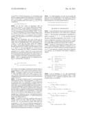
8. The method of claim 6, wherein determining a total minimum number of observable crossovers comprises: obtaining, for a pair of markers j and j', four counts, ck.sub.1.sub.k2, k1,k2=0,1 computed as: ck.sub.1.sub.k2=|{i|Mij=k1 and Mij=k2}| where the four counts in decreasing order are c.sup.1.gtoreq.c.sup.2.gtoreq.c.sup.3.gtoreq.c4 and Cij'={c1|1.ltoreq.l≦4}, and where for each j, jnxt is a smallest j'>j, where ΣcεCjj'c>0 and xo(j, jnxt)=c3+c4 and the total minimum number of observable crossovers is ≧Σj=1.sup.mxo(j, jnxt)=dc, and where l is an index.
9. The method of claim of 7, further comprising updating each Mijp≠X according to Vp and each Mijp=X based on M ij p { H if V j p ( 0 ) = V j p ( 1 ) , k else if V j p ~ ( k ) ≠ V j p ( k ) and V j p ~ ( 0 ) = V j p ~ ( 1 ) ##EQU00016## where, a pair of markers j and j' are polarized, and for the pair of markers j and j' a set of two counts c1 and c2 are one of c00 and c11 or c01 and c10, and if {c1, c2}={c01, c10}, then values Vj'(0) and Vj'(1) are updated by interchanging them.
10. The method of claim 9, further comprising: transforming each of the updated matrices Mijp to F(Ma) and F(Mb), respectively, using a set of monotonic state transitions based on functions Lt(Mij) and Rt(Mij), where Lt ( M ij ) = { k if M ij ' = k for 1 ≦ j ' < j , and there is no j ' < j '' < j with numeric M ij '' , - 1 otherwise Rt ( M ij ) = { k if M ij ' = k for j ≦ j ' < m , and there is no j ' > j '' > j with numeric M ij '' , - 1 otherwise ##EQU00017## where, for a fixed i, if {tilde over (F)}ij is not numeric but Fij is, Vj(0)=Vj(1) if {tilde over (F)}ij and Fij are both not numeric, then if, is a heterozygous trio, if Fij=-1, for some j, then Fij={tilde over (F)}ij=-1, for all j, and wherein F(Ma) and F(Mb) are constructed from Mija , and Mijb in O(mn) time.
11. The method of claim 10, wherein constructing the agglomerate data structure comprising the set of haplotype sequences comprises: generating an agglomerate of the set of haplotype sequences in a single pair of matrices Rijp, wherein p=a, b, from F(Ma) and F(Mb).
12. The method of claim 11, wherein Rijp is generated based on, for each progeny i: if Fij=-1 for some j, then Rij0 and {tilde over (R)}ij1, for all j; if Fijε{0,1}, then RijFij; for each j, if {tilde over (F)}ij is numeric and Fij is not, then Rijq; and for each j, where Fij and {tilde over (F)}ij are both not numeric, then R ij , R ~ ij { * if V j ( 0 ) = V j ( 1 ) , q if V j ( 0 ) ≠ V j ( 1 ) = V ~ j ( 0 ) & F ij ≠ F ~ ij , q if V j ( 0 ) ≠ V j ( 1 ) = V ~ j ( 1 ) & F ij = F ~ ij , Q otherwise ##EQU00018## where non-numeric values in Rijp encode multiple solutions.
13. The method of claim 12, wherein a switch sw occurs between q and Q, and between a numeric value adjacent to Q, where a number of switches in a non-numeric run r of Rijp is sw(r), and where for each non-numeric run r if sw(r)>0, then r begins and ends with Q and a position of a first switch and a position of a last switch are adjacent to the non-numeric run r.
14. The method of claim 13, where s=sw(r), and a total number of observable crossovers in the run r, across haplotypes from parent a and parent b, is exactly s and each observable crossover in each haplotype of the run r is at a position of a switch in the run r, and if r is an asymmetric run, s is zero.
15. The method of claim 13, further comprising: determining, for the collection of sets of haplotype sequences in the agglomerate data structure, a deviation, , from the total minimum number of observable crossovers in the n progenies as = r .di-elect cons. U sw ( r ) - 2 , ##EQU00019## where U is a set of all maximal non-numeric runs in R.
16. The method of claim 13, further comprising determining a measure of uncertainty, , of positions of observable crossovers in each run r of each set of haplotype sequences in the agglomerate data structure as = r .di-elect cons. U δ ( r ) ( m - 1 ) ( d c + ) , where ##EQU00020## δ ( r ) = { len ( r ) + 1 if sw ( r ) = 0 , l 2 c l otherwise ( c l is the wild card , and where count of each switch l in r ) ##EQU00020.2## a value of 0 indicates that a location of each observable crossover in the agglomerate data structure is known precisely, where a value of 1 indicates maximum uncertainty in the location, and where U is a set of all maximal non-numeric runs in R.
17. The method of claim 12, further comprising: determining an error estimate in as N/mn, where N is a number of genotype data mismatches in Rijp, where a position ij has a mismatch if {V(Rij),{tilde over (V)}({tilde over (R)}ij)}≠ij and Rij, {tilde over (R)}ijε{0,1}.
18. The method of claim of claim 12, further comprising: determining a haplotype frequency distribution for the collection of the set of haplotype sequences in the agglomerate data structure, wherein the determining is based on k1, k2=0,1 being a haplotype pair, and if Rij is non-numeric, let Rij=α hold, where for each marker j for x, y=0,1,α, cxy=|{i|Rija=x and Rijb=y}|, and an expected count ck.sub.1.sub.k2 of each haplotype pair is ck.sub.1.sub.k2=ck.sub.1.sub.k2+Δk.sub.1.s- ub.k2, where Δk.sub.1.sub.k2=c.sub.αk2/2+ck.sub.1.sub.- α/2+c.sub.αα/4.
19. The method of claim 18, further comprising: determining a variance σk.sub.1.sub.k.sub.2.sup.2 of haplotype frequency distribution as Δk.sub.1.sub.k.sub.2.
Description:
BACKGROUND
[0001] The present invention generally relates to the field of computational biology, and more particularly relates to exact haplotype reconstruction of F2 populations.
[0002] An important question when studying the genetics of an individual is that of determining its haplotype organization, i.e., determining the parental origin of each region in the individual's genome. When diploid organisms reproduce, crossovers frequently occur during meiosis. Therefore, progenies do not always receive complete copies of their parents' chromosomes. Instead, the genetic material inherited from a parent is often a combination of segments from the two chromosomes present in that parent, i.e. a combination of the two haplotypes of the parent (and similarly for material inherited from the other parent).
[0003] In practice, haplotypes are often constructed from genotype data. The genotype of an individual represents a sequence of unordered pairs of allele values associated with the diploid genome. Genotypes are often sampled as sequences of SNP (single-nucleotide polymorphism) marker values at locations spread across the genome. Determining the haplotypes for an individual at a given marker involves assigning each of the two unordered allele values to the correct parent from which it was inherited, and more precisely, to the correct haplotype of that parent.
[0004] Haplotype studies are extensively applied in the field of population genetics. For example, one can reconstruct so called ancestral founder haplotypes and represent the current population as a mosaic of those sequences. In another example, when the diploid parental genomes are known, one can separate them into haplotypes and represent the progenies as a mosaic of those haplotypes. The challenges of such applications include a) accurately collecting genomic data on the studied population, and b) constructing efficient and accurate algorithms for solving the associated combinatorially challenging problems.
BRIEF SUMMARY
[0005] In one embodiment, a method for reconstructing haplotypes from genotype data is disclosed. The method comprises accessing a set of progeny genotype data comprising n progenies encoded with m genetic markers. Each of the m genetic markers comprises two values per individual. Also, a combination of each of the m genetic markers associated with a progeny represents a genotype sequence of the progeny. A first set of parent haplotypes associated with a first parent of the n progenies and a second set of parent haplotypes associated with a second parent of the n progenies are identified based on at least the set of progeny genotype data. A total minimum number of observable crossovers in the n progenies is determined. An agglomerate data structure comprising a collection of sets of haplotype sequences characterizing the n progenies in terms of the first and second sets of parent haplotypes is constructed based on the set of progeny genotype data and the first and second sets of parent haplotypes. Each set of progeny haplotype sequences comprises a number of crossovers equal to the total minimum number of observable crossovers in the n progenies.
BRIEF DESCRIPTION OF THE SEVERAL VIEWS OF THE DRAWINGS
[0006] The accompanying figures where like reference numerals refer to identical or functionally similar elements throughout the separate views, and which together with the detailed description below are incorporated in and form part of the specification, serve to further illustrate various embodiments and to explain various principles and advantages all in accordance with the present invention, in which:
[0007] FIG. 1 is a block diagram illustrating one example of an operating environment according to one embodiment of the present invention;
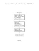
[0008] FIG. 2 is an illustrational flow of an overall process for reconstructing haplotypes from genotype data according to one embodiment of the present invention;
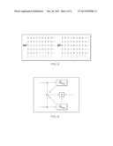
[0009] FIG. 3 illustrates one example of a matrix comprising genotype data according to one embodiment of the present invention;
[0010] FIG. 4 illustrates one example of parental encodings based on genotype data partially shown in FIG. 3 according to one embodiment of the present invention;
[0011] FIG. 5 shows one example of partially resolved haplotype sequences based on the encodings in FIG. 4 according to one embodiment of the present invention;
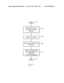
[0012] FIG. 6 illustrates permissible state transitions for haplotype matrices according to one embodiment of the present invention;
[0013] FIG. 7 is an operational flow diagram illustrating one example of a process for reconstructing haplotypes from genotype data according to one embodiment of the present invention; and
[0014] FIG. 8 is an operational flow diagram illustrating another example of a process for reconstructing haplotypes from genotype data according to one embodiment of the present invention.
DETAILED DESCRIPTION
[0015] Haplotype information can be extremely useful in determining the specific form of a gene that is associated with a phenotype such as disease susceptibility. Haplotype information can be used first to determine the genomic location of a gene associated with the phenotype and second to determine the exact forms (haplotypes) that are associated with the phenotype at that location. Haplotype information is also useful in the field of population genetics.
[0016] One problem with constructing haplotype information from genotype data is that given genotypes of n progenies on m loci, the general problem of constructing haplotypes from genotypes is NP complete under different models such as parsimony, maximum likelihood, and phylogeny. However, the duality of bi-allelic markers and F2 progenies (i.e., two founder sequences per haplotype), as is the case with plant breeding data, provides a compelling combinatoric puzzle. Rather than tweak generic software to adapt to the stringent conditions, embodiments of the present invention solve this problem more accurately and efficiently in a model-free setting. This is achieved, in one embodiment, by seeking out a mathematical lower bound on the number of crossovers in the data. The focus is not just on a maximum likely or a most parsimonious solution, but on an "agglomerate" of all (equally-likely) feasible solutions. All the computations including the agglomerate can be achieved in linear time. Also, the level of preciseness of the solution is such that it not only permits study of statistical trends, such as haplotype distributions along the chromosome, association with QTLs and so on, but can also help hand-pick individual recombinants that can be independently confirmed through resequencing for further experimentations.
OPERATING ENVIRONMENT
[0017] FIG. 1 illustrates a general overview of one operating environment 100 for reconstructing haplotypes according to one embodiment of the present invention. In particular, FIG. 1 illustrates an information processing system 102 that can be utilized in embodiments of the present invention. The information processing system 102 shown in FIG. 1 is only one example of a suitable system and is not intended to limit the scope of use or functionality of embodiments of the present invention described above. The information processing system 102 of FIG. 1 is capable of implementing and/or performing any of the functionality set forth above. Any suitably configured processing system can be used as the information processing system 102 in embodiments of the present invention.
[0018] As illustrated in FIG. 1, the information processing system 102 is in the form of a general-purpose computing device. The components of the information processing system 102 can include, but are not limited to, one or more processors or processing units 104, a system memory 106, and a bus 108 that couples various system components including the system memory 106 to the processor 104.
[0019] The bus 108 represents one or more of any of several types of bus structures, including a memory bus or memory controller, a peripheral bus, an accelerated graphics port, and a processor or local bus using any of a variety of bus architectures. By way of example, and not limitation, such architectures include Industry Standard Architecture (ISA) bus, Micro Channel Architecture (MCA) bus, Enhanced ISA (EISA) bus, Video Electronics Standards Association (VESA) local bus, and Peripheral Component Interconnects (PCI) bus.
[0020] The system memory 106, in one embodiment, comprises a reconstruction module 109 configured to reconstruct haplotypes of F2 populations. As will be discussed in greater detail below, the reconstruction module 109 takes as input a set of gentoypes of n F2 progenies on m markers. Based on this input the reconstruction module 109 extracts all the equally-likely haplotypes of the progenies to produce an agglomerate structure. This agglomerate structure can be utilized by the reconstruction module 109 to compute the parameters of the distribution of each individual crossover, which makes further analysis of haplotype frequencies both more informative as well as accurate. Additionally, the reconstruction module 109 can visualize the solutions (e.g., a collection of haplotype sequences satisfying a lower bound) as mosaics of the ancestor haplotypes. It should be noted that even though FIG. 1 shows the reconstruction module 109 residing in the main memory, the reconstruction module 109 can reside within the processor 104, be a separate hardware component, and/or be distributed across a plurality of information processing systems and/or processors.
[0021] The system memory 106 can include computer system readable media in the form of volatile memory, such as random access memory (RAM) 110 and/or cache memory 112. The information processing system 102 can further include other removable/non-removable, volatile/non-volatile computer system storage media. By way of example only, a storage system 114 can be provided for reading from and writing to a non-removable or removable, non-volatile media such as one or more solid state disks and/or magnetic media (typically called a "hard drive"). A magnetic disk drive for reading from and writing to a removable, non-volatile magnetic disk (e.g., a "floppy disk"), and an optical disk drive for reading from or writing to a removable, non-volatile optical disk such as a CD-ROM, DVD-ROM or other optical media can be provided. In such instances, each can be connected to the bus 108 by one or more data media interfaces. The memory 106 can include at least one program product having a set of program modules that are configured to carry out the functions of an embodiment of the present invention.
[0022] Program/utility 116, having a set of program modules 118, may be stored in memory 106 by way of example, and not limitation, as well as an operating system, one or more application programs, other program modules, and program data. Each of the operating system, one or more application programs, other program modules, and program data or some combination thereof, may include an implementation of a networking environment. Program modules 118 generally carry out the functions and/or methodologies of embodiments of the present invention.
[0023] The information processing system 102 can also communicate with one or more external devices 120 such as a keyboard, a pointing device, a display 122, etc.; one or more devices that enable a user to interact with the information processing system 102; and/or any devices (e.g., network card, modem, etc.) that enable computer system/server 102 to communicate with one or more other computing devices. Such communication can occur via I/O interfaces 124. Still yet, the information processing system 102 can communicate with one or more networks such as a local area network (LAN), a general wide area network (WAN), and/or a public network (e.g., the Internet) via network adapter 126. As depicted, the network adapter 126 communicates with the other components of information processing system 102 via the bus 108. Other hardware and/or software components can also be used in conjunction with the information processing system 102. Examples include, but are not limited to: microcode, device drivers, redundant processing units, external disk drive arrays, RAID systems, tape drives, and data archival storage systems.
HAPLOTYPE RECONSTRUCTION
[0024] As discussed above, the reconstruction module 109 reconstructs haplotypes of F2 (the second filial generation resulting from the cross-mating or self-mating of a first filial generation) progenies in a set of genotypes. FIG. 2 shows an overview of this haplotype reconstruction process. For example, FIG. 2 shows that the reconstruction module 109 receives a genotype matrix as input. The reconstruction module 109 constructs haplotype matrices M from and identifies the column j where exactly one of parent haplotypes Va and Vb is homozygous (i.e., two identical alleles exist at a given locus). The identified columns are resolved (based on Observation 3 discussed below) to identify a set of markers with exactly one heterozygous (i.e., two different alleles exist at a given locus) parent p. The matrices M are updated (based on EQ. 2 discussed below) and each of the parental haplotype pairs Va and Vb are phased (based on Observation 4 discussed below), where phasing denotes resolving the haplotypes. State transitions are used to construct a unique matrices F from matrices M (based on observations 6 and 7 discussed below). An agglomerate structure R (i.e., matrices Ra and Rb) is created from matrices F and runs r in R are processed (based on observation 8 discussed below). The reconstruction module 109 then outputs all equally-likely solutions (a collection of haplotype sequence sets, comprising each progeny in the genotype data, that satisfy a lower bound) based on observations 9 and 10 discussed below. The reconstruction module 109 also outputs haplotype distributions (based on observation 11 discussed below).
[0025] The following is a more detailed discussion on the haplotype reconstruction process shown in FIG. 2. In one embodiment the set of genotype data is structured within a matrix , as shown in FIG. 3. Matrix is an n×m matrix that encodes n progenies with m markers. Each row i, 1≦i≦n , represents a progeny and each column j, 1≦j≦m, represents a marker. The order of the markers is also captured in the matrix, i.e., j'<j<j'' if and only if marker j is located between markers j' and j'' on the chromosome. A marker j is polymorphic if there exist progenies i≠i', such that ij≠ij. In one embodiment, all the markers in are considered to be polymorphic.
[0026] The jth marker of the ith progeny, also referred to as the position ij, is ij which is a pair of SNPs (single-nucleotide polymorphisms), or alternatively a pair of any other genomic markers with two possible values per position. Each individual SNP can be accessed as ij(0) and ij(1). Thus if ij={A,C} or simply written as AC, ij(0)=A and ij(1)=C. When ij(0)=ij(1), the position ij is said to be homozygous. Similarly, when ij(0)≠ij(1), the position ij is said to be heterozygous.
[0027] If dt is the true number of crossovers, then 0≦dt≦2(m-1)n and an estimate dc≦0 is a lower bound of dt, if it is no larger than dt. Consider a scenario where each position ij in is heterozygous. In this case, the theoretical lower bound, on the number of crossovers in the unknown haplotypes of the progenies, is zero. Also there exists an exponentially large number (2mn) of distinct equally-likely haplotype configurations of the progenies each with no crossover. While informative markers in general are chosen for their heterozygosity in data sets, it is observed that the same marker is also homozygous in many a progeny. Thus, in one embodiment, due to Mendelian inheritance, it is very unlikely to have a run of markers that are heterozygous in all the progenies. It is this random sprinkling of homozygous positions in that makes estimation of a non-trivial lower bound possible.
[0028] Simulations were conducted to study the relationship between the lower bound estimate dc and extent of homozygosity in in realistic data scenarios. For an algorithm-independent estimation of dc the following criteria was used for detectable crossovers. Let run r between ij and ij be the sequence of entries of in the row i, between columns j to j'. Further, r is a heterogenous run if it contains both homozygous and non-homozygous values. For progeny i, let j1<j2 be such that there is no crossover at ij where j1<j<j2 and at least one of ij1 and ij2 is a crossover position. Without loss of generality let j1 be a position of crossover, then the crossover at ij1 is considered detectable if the run between ij1 and ij2 is heterogenous. Then the total number of detectable crossovers is dc, the estimate on the lower bound.
[0029] Let e denote the mean number of crossovers in a progeny. Simulations were used with values 2≦e≦15. It was observed that for this wide range of crossover profiles, the required fraction of homozygous sites in to get a good estimate of dt (i.e., within 5% of the true value) was fixed. The empirical observation is summarized as follows: (Observation 1) When at least 28% of each subsample of randomly chosen positions in is homozygous, the estimated lower bound dc is within 5% of the exact value dt, i.e., dc≧0.95dt.
[0030] In practice, values of n in the range of 50 to 400 and m in the range of 30 to 600 can be encountered. It has been consistently observed that at least 50% of the positions are homozygous and the solutions, obtained using methods discussed below, displayed e≈2. With a decrease in cost and an increase in accessibility of sequencing and genotyping technologies, m can be orders of magnitude larger in the near future. Note that e is not expected to increase with m . Thus, the lower bound estimation scales well with m, since the observation above is independent of m and the algorithm discussed in the later sections is linear in m.
[0031] Since each marker is bi-allelic, each column in has no more than two distinct values. This can be seen in each column of the matrix shown in FIG. 3. Furthermore, the marker at each (yet unknown) haplotype of the progeny has two possible values. Let the two parents be denoted as a and b. Then the two distinct SNP values of parent p are represented by Vjp(0) and Vjb(1), p=a,b. Let Z and Z' be the two SNP values seen in the column j of , written as ={Z, Z'}. Then if Z=Z' then Va(k)=Vb(k), for k=0,1. Let Z≠Z'. If there exists a progeny i with homozygous SNP Z, i.e., ij=ZZ, then Vja(0)=Vjb(0)=Z. If there also exists some i'≠i such that ij=Z'Z'Z', then Vja(1)=Vjb(1)=Z'. Note that if there is no such i' then only one of Va(1) and Vb(1) is Z' and the other is Z. Based on this, is separated naturally into two matrices Ma and Mb. For each i and j, and p=a,b.
M ij p = { k if ij ( 0 ) = V j p ( k ) , X if . ( EQ . 1 ) ##EQU00001##
[0032] When each haplotype is expected to have exactly two founders then a represents one parent and b the other. This condition holds when all the progenies are crossed from exactly one pair of parents. In particular, for a crossed population, Va(0) encodes haplotype 0 of parent a and Va(1) encodes haplotype 1 of parent a. Similarly, Vb(0) and Vb(1). A lower bound computation also phases the parents a and b, through the appropriate updating of Vp, p=a,b.
[0033] FIG. 4 shows one example of Va and Vb encodings based on the genotype data of FIG. 3. As can be seen, Va and Vb are encoded to indicate the markers where each parent is heterozygous (X), where only one parent is heterozygous (x or x'), where one parent is homozygous (H), and where both parents are homozygous (h).
[0034] Let conjugate of z be written as {tilde over (z)}, where z is a matrix or a discrete value as defined below. Note that the conjugate of conjugate of z is z, i.e., z= always holds. For parents p=a,b, if p=a, then {tilde over (p)}=b and vice-versa. Similarly, if k=0, then {tilde over (k)}=1 and vice-versa. Thus Ma={tilde over (M)}b (and Mb={tilde over (M)}a). Also, {tilde over (V)}p(0)=Vp(1) and {tilde over (V)}p(1)=Vp(0) for the parents p=a,b. It should be noted that for readability purposes the superscript a (or b) from Ma and Va (or Mb and Vb) is removed wherever unambiguous. For a pair of markers j and j' four counts, ck1k2, k1,k2=0,1 are computed as:
ck1k2=|{i|Mij=k1 and Mij'=k2}|.
[0035] Let the four counts in decreasing order be c1≧c2≧c3≧c4 and let Cjj'={c1|1≦1≦4}. Without loss of generality, for each j, let jnxt be the smallest j'>j such that ΣcεCjj'c>0. Let xo(j, jnxt)=c3+c4. In fact, the minimal number of crossovers (or recombinations) between marker j and jnxt is xo(j, jnxt). Moreover, the following is easily verified: (Observation 2) Given genotype data on n progenies with m bi-allelic markers, the total number of crossovers in the progenies is ≧Σj=1mxo(j, jnxt)=dc.
[0036] In one embodiment, the lower bound can be improved by using appropriate threshold values at different stages. Thus, for a threshold, thrsh1=0.3 n, the marker jnxt for a given j is such that the counts satisfy the condition Σc1>thrsh1. This modified definition where j'=jnxt is used in the following discussion. Further, when the quartet of counts c1, c2 and c3, c4 are well separated, i.e., (c3+c4)/(c1+c2)<thrsh2, say with thrsh2=0.15 , then Cjj' is referred to as being polarized. Let j={Z≠Z'}. Then Vjp(1), p=a,b, can be computed based on the following observation: (Observation 3) If Cjj' is not polarized, then jεJp and j'εJ.sub.{tilde over (p)}, for some p, where Jp is the set of markers with exactly one heterozygous parent p.
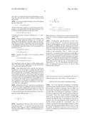
[0037] After Vp is updated each Mijp≠X is updated according to Vp and each Mijp=X based on
M ij p { H if V j p ( 0 ) = V j p ( 1 ) , k else if V j p ~ ( k ) ≠ V j p ( k ) and V j p ~ ( 0 ) = V j p ~ ( 1 ) ( EQ . 2 ) ##EQU00002##
FIG. 5 shows one example of matrices Ma and Mb based on the encodings in Va and Vb shown in FIG. 4 and EQ. 2 above.
[0038] For the pair of markers j and j', the two larger values (c1 and c2) are either c00 and c11 or c01 and c10. If {c1,c2}={c01,c10}, then the values Vj'(0) and Vj'(1) are updated by interchanging them. Recall that the number of crossovers between j and j' is ≧(c3+c4).
[0039] For the pair of markers j and j', Cjj' must be polarized (Observation 4). Hence, when the quartet c1, c2 and c3, c4 is not polarized, then it is reasonable to assume significant experimental errors in the genotyping of marker j' (or j). To ensure that Vj' is not updated multiple times, the reconstruction module 109 begins with the leftmost j where both Vj are not homozygous. The marker j' is picked as above and then at the next stage j is assigned j' and the process continued until all j have been handled. In one embodiment, j' on the other side of j can be selected, while taking care not to update Vj' multiple times. Furthermore, given , the haplotype matrices Ma,Mb and the parent haplotypes Va, Vb can be constructed in O(mn) time (Observation 5).
[0040] It should be noted that sometimes there may be missing values in the data. When the value is missing at position ij, the reconstruction module 109 makes the assignment ijXX. However, if after the computation of V, marker j is homozygous at parent p, then MijpH and Mij.sup.{tilde over (p)} is appropriately updated. It can be verified that this treatment ensures that the estimated lower bound, dc, is unaltered.
[0041] For selfed progenies, not only are the parents the same but even the haplotypes of the parents are deemed identical. Given selfed progenies, one of the following conditions holds for p=a,b and a numeric kε{0,1}:
Va=Vb and if Mijp=k then Mij.sup.{tilde over (p)}={tilde over (k)}, for all i and j, or, (1)
Va≠Vb and if Mijp=k then Mij.sup.{tilde over (p)}=k, for all i and j. (2)
MEASURE OF UNCERTAINTY
[0042] In one embodiment, the reconstruction module 109 determines the preciseness of the output given a genotype matrix . This preciseness measurement is quantified by a triplet of measures , , . is the deviation from the theoretical (algorithm-independent) lower bound. is the extent of dispersion in position of each crossover. is the error in the data. To compute these measures the reconstruction module 109 transforms the matrices Mp as follows.
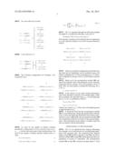
[0043] A parent, p, is homozygous at marker j when Vjp(0)=Vjp(1) and is heterozygous otherwise. A position ij is a heterozygous trio, if the two parents at j are heterozygous and so is ij. Let k represent a numeric value and two functions Lt() and Rt() on an element of the matrix is defined as follows:
Lt ( M ij ) = { k if M ij ' = k for 1 ≦ j ' < j , and there is no j ' < j '' < j with numeric M ij '' , - 1 otherwise . Rt ( M ij ) = { k if M ij ' = k for j ≦ j ' < m , and there is no j ' > j '' > j with numeric M ij '' , - 1 otherwise . ##EQU00003##
[0044] A set of transitions, S_→S_ that systematically transform the elements of M is now defined. Let Mij=x. Then the transition Sx→S_ is applied to assign the value y to Mij (written as Mijy) as follows.
• S H -> S e k , S X -> S e k ##EQU00004## If Lt ( M ij ) = Rt ( M ij ) = k , then M ij e k . • S H -> S w k 1 k 2 H , S X -> S w k 1 k 2 X ##EQU00004.2## If Lt ( M ij ) ≠ Rt ( M ij ) with Lt ( M ij ) = k 1 and Rt ( M ij ) = k 2 , then M ij w k 1 k 2 . • S w k 1 k 2 X -> S e k , S w k 1 k 2 H -> S e k ( note that k 1 ≠ k 2 ) ##EQU00004.3## If Lt ( M ij ) = Rt ( M ij ) = k , then M ij e k . • S e k -> S k ##EQU00004.4## M ij k . • S w k 1 k 2 X -> S k ##EQU00004.5## If M ~ ij is numeric , then M ij V ~ ( M ~ ij ) . ##EQU00004.6##
[0045] In the above transitions ek is a temporary value in matrix M that is not present in the final version of M (i.e., matrix F discussed below). For example, e0 at Mij denotes the case where the closest numerical value to the left and right of Mij is 0 (i.e. haplotype 0 spans over this marker at individual i). Eventually ek is stored as k in Mij [in the Sek→Sk transition]. Also, wk1k2 is a non-numerical value that can occur in the M and F matrices. The possible values are w01 and w10. For example, w01 at Mij represents the case where the closest numerical value to the left of Mij is 0 and the closest numerical value to the right is 1 (there is a crossover at individual i whose location could be j). The values wk1k2 are considered in steps 3 and 4 (as non-numerical values in F) discussed below with respect to the agglomerate solution R.
[0046] To estimate the running time of the algorithm, the transitions are classified as intra-transitions and inter-transitions, depending on whether M or {tilde over (M)} is used respectively. Thus,
S w k 1 k 2 X -> S k ##EQU00005##
is the only inter-transition. The above transitions are applied to the elements of Ma and Mb till no more transition is applicable. This final form of matrix is written as F(Ma) or simply Fa. Similarly, F(Mb) or simply Fb. The permissible transitions are captured in the transition diagram shown in FIG. 6. The three possible start states are SH, SX and Sk, and the three possible final states are shown in boxes. The curly arrow represents the inter-transition while the straight arrows represent the intra-transitions. Note that each Mij undergoes no more than three transitions since there are no cycles in the state transition diagram. Also, each state with multiple outgoing edges has non-overlapping conditions, leading to a unique choice of transition.
[0047] Each element of Fp is in the final state, i.e., for each position ij), Fijpε{0,1, w01, w10, -1}, p=a,b. A numeric value of -1 indicates that no information regarding the haplotypes can be deduced. The state transitions induce the following properties on F and V: (Observation 6) For a fixed i, the following hold:
If {tilde over (F)}ij is not numeric but Fij is, then Vj(0)=Vj(1) must hold. (1)
If {tilde over (F)}ij and Fij are both not numeric, then ij, must be a heterozygous trio. The converse however is not true. (2)
If Fij=-1, for some j, then Fij={tilde over (F)}ij=-1, for all j. (3)
(Observation 7)
[0048] Given Ma and Mb, Fa and Fb are unique. (1)
Fa and Fb can be constructed from Ma and Mb in O(mn) time. (2)
[0049] To show that Fa and Fb are unique, the iterations can be viewed as of two types: one where only inter-transitions and the other where only intra-transitions are applicable. In the very first iteration, due to the possible start states, no inter-transition can be applied. In the second iteration, where no intra-transition can be applied, the uniquely applicable inter-transitions are applied. Thus the iterations alternate between intra- and inter-transitions. Hence the final forms Fa and Fb are unique. Next, since each entry can go through no more than three transitions, it is possible to obtain Fa and Fb from Ma and Mb in O(mn) time using suitable list data structures.
[0050] With respect to the agglomerate of feasible solutions, suppose there are L>0 feasible distinct solutions for a given . The reconstruction module 109, in one embodiment, generates an agglomerate in a single pair of matrices Ra and Rb that captures all the L solutions. The following illustrates one embodiment how the reconstruction module 109 constructs the agglomerate (Ra and Rb) based on the encodings in Fa and Fb discussed above.
[0051] Let the conjugate of F be {tilde over (F)} defined as {tilde over (F)}a=Fb and {tilde over (F)}b=Fa. Rijp that encodes all the possible solutions, is constructed from Fijp, p=a,b, as follows. New symbols *, q and Q are used in addition to the numeric values (0 and 1) in R. Also, for readability purposes the superscript a and b is removed, wherever unambiguous. For each progeny i:
[0052] 1. If Fij=-1 for some j, then without loss of generality Rij0 and {tilde over (R)}ij1, for all j.
[0053] 2. If Fijε{0,1}, then RijFij.
[0054] 3. For each j, if {tilde over (F)}ij is numeric and Fij is not, then Rijq.
[0055] 4. For each j, where Fij and {tilde over (F)}ij are both not numeric, then
[0055] R ij , R ~ ij { * if V j ( 0 ) = V j ( 1 ) , q if V j ( 0 ) ≠ V j ( 1 ) = V ~ j ( 0 ) & F ij ≠ F ~ ij , q if V j ( 0 ) ≠ V j ( 1 ) = V ~ j ( 1 ) & F ij = F ~ ij , Q otherwise . ##EQU00006##
The non-numeric values in R encode multiple solutions, possibly with multiple crossovers, as discussed below.
[0056] With respect to the deviation from the lower bound dc, let r be a run of contiguous values in a row (progeny) of R. Further, let r be maximal i.e., if r is non-numeric then it must be sandwiched on both sides by numeric values. Stated differently, if r is non-numeric the first and last non-numeric values of r are adjacent to a numeric value. Let ra and rb be the non-numeric runs in the two haplotypes of the progeny and are aligned in the examples discussed below. It is possible that only one of ra or rb is a numeric run, and this run is referred to as asymmetric. However, if both are non-numeric, then by construction ra=rb and the run is symmetric. In the following discussion, the superscripts are removed, wherever unambiguous, for readability purposes.
[0057] A switch is defined to occur between q and Q or between Q and the numeric value that sandwiches the run. The number of switches is written as sw(r). The switch detection performed by the reconstruction module 109 is described by the following two examples. In the examples shown below, the run is represented by the non-numeric values in bold with numeric values to the left and right of the run. Each switch is marked as a numbered down-arrow.
[0058] In a first example (Example 1) consider the following run:
r=ra=rb= . . . 000qqQQqqQQ111 . . .
The number of switches is 4 as shown:
. . . 000qq↓1QQ↓2qq↓3QQ↓4111 . . .
The value * is a wild card and can be treated either as q or Q. Thus, the wild card may result in different positions of the same switch.
[0059] In a second example (Example 2) the following run has three wild cards:
r=ra=rb= . . . 000q*qQ*QQqq*Q111 . . .
The first wild card is treated as a q, the second wild card is treated as a Q, and the third wild card can be treated as a q or Q with two possible positions for the third switch.
. . . 000q*q↓1Q*QQ↓2qq↓3*↓.su- b.3'Q↓4111 . . .
The wild card counts of the four switches are 1, 1, 2, and 1 respectively.
[0060] When sw(r)>0, the location of the switches in the run r may define additional positions ij in R that can updated from non-numeric to numeric. These are the positions that are to the left of the leftmost switch and to the right of the rightmost switch positions. Thus, the run of Example 1 is transformed where the length of the non-numeric run shrinks from 8 to 6.
. . . 000qq↓1QQ↓2qq↓3QQ↓- 4111 . . .
. . . 00000↓1QQ↓2qq↓3QQ↓4111 . . .
[0061] Similarly the length of run of Example 2 shrinks from 11 to 9.
. . . 000q*q↓1Q*QQ↓2qq↓3*↓.su- b.3'Qred↓4. . .
. . . 000000↓1Q*QQ↓2qqd↓3*↓.s- ub.3'Q↓4111 . . .
The transformed values are shown in bold numeric values above. The same process is applied to every non-numeric run r to transform the matrices Ra and Rb.
[0062] Then (Observation 8) R is such that for each non-numeric run r, if sw(r)>0, then (1) r begins and ends with Q and (2) the positions of the first and the last switch sandwich the non-numeric run. To summarize: (Observation 9) Let r be a non-numeric run and let s=sw(r). Then (1) the total number of crossovers in the run, across both the haplotypes, is exactly s and each crossover in each haplotype of the configuration is at a position of the switch. (2) If r is an asymmetric run, s is zero. In general, s is even and the number of crossovers in each haplotype of each distinct configuration is odd. However, is this not a requirement.
[0063] (Observation 10) Let s=sw(r) for a non-numeric run r. Then if s≦2, there is no additional crossover introduced by r. If s>2, the number of additional crossovers is s-2. Let U be the set of all maximal non-numeric runs in R. Then if denotes the deviation from the lower bound, dc, the reconstruction module 109 calculates as
= r .di-elect cons. U sw ( r ) - 2 . ##EQU00007##
[0064] Regarding the dispersion index and error estimate, the dispersion index, , is a measure of the uncertainty in the position of the crossovers. This is computed by the reconstruction module 109 as an average over all predicted crossovers. Thus,
= r .di-elect cons. U δ ( r ) ( m - 1 ) ( d c + ) , where ##EQU00008## δ ( r ) = { len ( r ) + 1 if sw ( r ) = 0 , l 2 c l otherwise ( c l is the wild card count of each switch l in r ) . ##EQU00008.2##
When the location of each crossover is known precisely, this index is 0. A value of 1 indicates maximum uncertainty in the location.
[0065] If Rij,{tilde over (R)}ijε{0,1}, then the position ij has a mismatch if {V(Rij),{tilde over (V)}({tilde over (R)}ij)}≠. Note that the mismatch at this position could be flagged as an error or one of Rij and {tilde over (R)}ij can be modified to potentially introduce additional crossover(s). These are undetectable during the lower bound computation and do not overlap with the non-numeric regions. Let N be the number of such mismatches. Then, , which is the error estimate in calculated by the reconstruction module 109, is defined as N/mn. In most instances the number of mismatches is very low (less than 0.01%) and the mismatches are experimental errors. Hence, the convention that such a mismatch be flagged as a potential error has been followed in one embodiment. Then, an error, if any, is at ij in F that underwent the transitions SX→. . . Sek→Sk. Note that the converse is not true. Also, an additional crossover, if any, is at ij in F that underwent the transitions
S X -> S w k 1 k 2 X . ##EQU00009##
Again, the converse is not true. To summarize, the trio () define the uncertainty in the solution of the genotypes .
HAPLOTYPE FREQUENCY DISTRIBUTIONS
[0066] One of the important consequences of haplotype inferencing is the haplotype frequency distribution across the chromosomes. A marker j of progeny i has two SNPs, one derived either from haplotype 0 or haplotype 1 of parent a and the other either from haplotype 0 or haplotype 1 of parent b. Since R is an agglomerate data structure and also contains the non-numeric values that encode multiple configurations. Based on the encoding in R the reconstruction module 109 estimates the expected value of the frequency count and its variance. First, the reconstruction module enumerates the feasible solutions encoded by a non-numeric run r. For example, consider the following example (Example 3) where in each of the following the length of the run, len(r), is 3 and the number of additional crossovers is zero. However, the number of configurations is different based on the structure of the switches.
[0067] Two runs with sw(r)=0 each:
r a = 00 qqq 111 r b = 11 qqq 000 or r a = 00 ** * 111 r b = 11 ** * 000 ⇄ { 00 111111 11 000000 or 000 11111 111 00000 or 0000 1111 11111 0000 or 00000 111 11111 000 ##EQU00010##
[0068] A run with sw(r)=2:
r a = 00 QQQ 111 r b = 11 QQQ 000 00 ↓ 1 QQQ ↓ 2 111 } ⇄ { 00 1 111111 11111 2 000 or 11111 2 000 00 1 111111 ##EQU00011##
[0069] The 8 distinct configurations for Example 1 discussed above are:
or 00000 1 111111111 0000000 2 11 3 00 4 111 0000000 2 11 3 00 4 111 00000 1 111111111 or or 0000000 2 1111111 00000 1 1111 3 00 4 111 00000 1 1111 3 00 4 111 0000000 2 1111111 or or 000000000 3 11111 00000 1 11 2 0000 4 111 00000 1 11 2 0000 4 111 000000000 3 11111 or or 00000000000 4 111 00000 1 11 2 00 3 11111 00000 1 11 2 00 4 11111 00000000000 4 111 ##EQU00012##
[0070] Let wt(r) be the number of distinct solutions encoded by r. (Observation 11) Let s=sw(r) for a run r. Let c1, c2, . . . cs be the wild card counts of the switch positions. Let wt(r) be the number of distinct feasible solutions due to r. Then
If s<2, wt(r)=len(r)+1. (1)
If s≧2, wt(r)=Z(r)Πl=1sc1, where (2)
Z ( r ) = 2 ( l = 1 s / 4 - 1 ( s 2 l - 1 ) ) + ( s 2 [ s / 4 ] - 1 ) . ( EQ . 3 ) ##EQU00013##
[0071] EQ. 3 is explained through the following example (Example 4). Consider the following r with sw(r)=6:
000QqQqQ111000↓1Q↓2q↓3Q↓4q↓5Q↓6111
Note that the 6 switches can be shared by the two haplotypes as 1 and 5 (the first column), or as 3 and 3 (second column) as follows.
000 1 11111111 000 1 1 2 0 3 11111 0000 2 1 3 0 4 1 5 0 6 111 000000 4 1 5 0 6 111 or or 0000 2 1111111 000 1 111 4 00 6 111 000 1 11 3 0 4 1 5 0 6 111 0000 2 1 3 00 5 1111 or or ##EQU00014##
[0072] There are six distinct configurations for the first case and since the two haplotypes can be switched it gives 2×6 distinct configurations. For the second there are (36)=20 distinct configuration, giving a total of 12+20 distinct solutions due to r.
[0073] Based on R, the reconstruction module 109 estimates the expected value of the frequency count of the haplotype pairs and its variance. If Rij is non-numeric, let Rij=α hold. Thus, for each marker j consider the following, for x, y=0,1, α,
cxy=|{i|Rija=x and Rijb=y}|
[0074] In the absence of any other external information, each of the alternative solutions in R is equally likely. Under this assumption, the expected count, ck1k2, of each haplotype pair, k1, k2=0,1, is estimated as follows:
cck1k2ck1k2+Δk1.- sub.k2, where
Δk1k2=c.sub.αk2/2+ck1.sub..alp- ha./2+c.sub.αα/4.
Further, the variance σk1k22 of the count of the haplotype pair is approximated as Δk1k2.
[0075] It should be noted that the reconstruction module 109, in one embodiment, outputs the equally-likely solutions in R as well as the haplotype distribution and variance information to a user. Additionally, the reconstruction module 109 can visualize the solutions as mosaics of the ancestor haplotypes. This information can be output to a display where the user can interact with the information.
OPERATIONAL FLOW DIAGRAMS
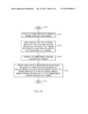
[0076] FIG. 7 is an operational flow diagram illustrating one example of an overall process for reconstructing haplotypes from genotype data. The operational flow diagram begins at step 702 and flows directly to step 704. The reconstruction module 109, at step 704, obtains genotype data on a population of several F2 individuals. The reconstruction module 109, at step 706, constructs an input matrix from the genotype data. The reconstruction module 109, at step 708, performs the haplotype reconstruction operations discussed above. The reconstruction module 109, at step 710, outputs all equally-likely solutions along with an uncertainty measure (i.e. a preciseness of the agglomerate data structure in terms of statistical measures) and haplotype distributions. This information can be used to study statistical trends such as haplotype distribution along chromosomes to, for example, observe biases. This information can also be used to hand-pick individuals based on their observed recombinations for further examination. It should be noted that other analyses can be performed on this information as well. The control flow exits at step 712.
[0077] FIG. 8 is an operational flow diagram illustrating another example of a process for reconstructing haplotypes from genotype data. The operational flow diagram begins at step 802 and flows directly to step 804. The reconstruction module 109, at step 804, accesses a set of progeny genotype data comprising n progenies encoded with m genetic markers. Each of the m genetic markers comprises two values. Also, a combination of each of the m genetic markers associated with a progeny represents a genotype sequence of the progeny. The reconstruction module 109, at step 806, identifies, based on at least the set of progeny genotype data, a first set of parent haplotypes associated with a first parent of the n progenies and a second set of parent haplotypes associated with a second parent of the n progenies. The reconstruction module 109, at step 808, determines a total minimum number of observable crossovers in the n progenies. The reconstruction module 109, at step 810, constructs, based on the set of progeny genotype data and the first and second sets of parent haplotypes, an agglomerate data structure comprising a collection of a set of haplotype sequences characterizing the n progenies in terms of the first and second sets of parent haplotypes. Each set of haplotype sequences comprises a number of observable crossovers equal to the total minimum number of observable crossovers in the n progenies. The control flow exits at step 812.
NON-LIMITING EXAMPLES
[0078] As will be appreciated by one skilled in the art, aspects of the present invention may be embodied as a system, method, or computer program product. Accordingly, aspects of the present invention may take the form of an entirely hardware embodiment, an entirely software embodiment (including firmware, resident software, micro-code, etc.) or an embodiment combining software and hardware aspects that may all generally be referred to herein as a "circuit," "module" or "system." Furthermore, aspects of the present invention may take the form of a computer program product embodied in one or more computer readable medium(s) having computer readable program code embodied thereon.
[0079] Any combination of one or more computer readable medium(s) may be utilized. The computer readable medium may be a computer readable signal medium or a computer readable storage medium. A computer readable storage medium may be, for example, but not limited to, an electronic, magnetic, optical, electromagnetic, infrared, or semiconductor system, apparatus, or device, or any suitable combination of the foregoing. More specific examples (a non-exhaustive list) of the computer readable storage medium would include the following: an electrical connection having one or more wires, a portable computer diskette, a hard disk, a random access memory (RAM), a read-only memory (ROM), an erasable programmable read-only memory (EPROM or Flash memory), an optical fiber, a portable compact disc read-only memory (CD-ROM), an optical storage device, a magnetic storage device, or any suitable combination of the foregoing. In the context of this document, a computer readable storage medium may be any tangible medium that can contain, or store a program for use by or in connection with an instruction execution system, apparatus, or device.
[0080] A computer readable signal medium may include a propagated data signal with computer readable program code embodied therein, for example, in baseband or as part of a carrier wave. Such a propagated signal may take any of a variety of forms, including, but not limited to, electro-magnetic, optical, or any suitable combination thereof. A computer readable signal medium may be any computer readable medium that is not a computer readable storage medium and that can communicate, propagate, or transport a program for use by or in connection with an instruction execution system, apparatus, or device.
[0081] Program code embodied on a computer readable medium may be transmitted using any appropriate medium, including but not limited to wireless, wireline, optical fiber cable, RF, etc., or any suitable combination of the foregoing.
[0082] Computer program code for carrying out operations for aspects of the present invention may be written in any combination of one or more programming languages, including an object oriented programming language such as Java, Smalltalk, C++ or the like and conventional procedural programming languages, such as the "C" programming language or similar programming languages. The program code may execute entirely on the user's computer, partly on the user's computer, as a stand-alone software package, partly on the user's computer and partly on a remote computer or entirely on the remote computer or server. In the latter scenario, the remote computer may be connected to the user's computer through any type of network, including a local area network (LAN) or a wide area network (WAN), or the connection may be made to an external computer (for example, through the Internet using an Internet Service Provider).
[0083] Aspects of the present invention have been discussed above with reference to flowchart illustrations and/or block diagrams of methods, apparatus (systems) and computer program products according to various embodiments of the invention. It will be understood that each block of the flowchart illustrations and/or block diagrams, and combinations of blocks in the flowchart illustrations and/or block diagrams, can be implemented by computer program instructions. These computer program instructions may be provided to a processor of a general purpose computer, special purpose computer, or other programmable data processing apparatus to produce a machine, such that the instructions, which execute via the processor of the computer or other programmable data processing apparatus, create means for implementing the functions/acts specified in the flowchart and/or block diagram block or blocks.
[0084] These computer program instructions may also be stored in a computer readable medium that can direct a computer, other programmable data processing apparatus, or other devices to function in a particular manner, such that the instructions stored in the computer readable medium produce an article of manufacture including instructions which implement the function/act specified in the flowchart and/or block diagram block or blocks.
[0085] The computer program instructions may also be loaded onto a computer, other programmable data processing apparatus, or other devices to cause a series of operational steps to be performed on the computer, other programmable apparatus or other devices to produce a computer implemented process such that the instructions which execute on the computer or other programmable apparatus provide processes for implementing the functions/acts specified in the flowchart and/or block diagram block or blocks.
[0086] The terminology used herein is for the purpose of describing particular embodiments only and is not intended to be limiting of the invention. As used herein, the singular forms "a", "an" and "the" are intended to include the plural forms as well, unless the context clearly indicates otherwise. It will be further understood that the terms "comprises" and/or "comprising," when used in this specification, specify the presence of stated features, integers, steps, operations, elements, and/or components, but do not preclude the presence or addition of one or more other features, integers, steps, operations, elements, components, and/or groups thereof.
[0087] The description of the present invention has been presented for purposes of illustration and description, but is not intended to be exhaustive or limited to the invention in the form disclosed. Many modifications and variations will be apparent to those of ordinary skill in the art without departing from the scope and spirit of the invention. The embodiment was chosen and described in order to best explain the principles of the invention and the practical application, and to enable others of ordinary skill in the art to understand the invention for various embodiments with various modifications as are suited to the particular use contemplated.
User Contributions:
Comment about this patent or add new information about this topic:
| People who visited this patent also read: | |
| Patent application number | Title |
|---|---|
| 20210155937 | COMPOSITIONS AND METHODS FOR INHIBITING EXPRESSION OF CD274/PD-L1 GENE |
| 20210155936 | MODULATION OF GENE EXPRESSION AND SCREENING FOR DEREGULATED PROTEIN EXPRESSION |
| 20210155935 | MODULATORS OF EZH2 EXPRESSION |
| 20210155934 | ANTISENSE ANTIBACTERIAL COMPOUNDS AND METHODS |
| 20210155933 | TLR-9 AGONISTS FOR MODULATION OF TUMOR MICROENVIRONMENT |
Images included with this patent application:
 |  |
 |  |
 |  |
 |  |
 |  |
| Similar patent applications: | |
| Date | Title |
|---|---|
| 2014-06-19 | Multi-posture stride length calibration system and method for indoor positioning |
| 2014-06-19 | Method for characterization of accumulators and related devices |
| 2014-06-19 | Determining a value of a variable on an rf transmission model |
| 2014-06-19 | Location change detection based on ambient sensor data |
| 2012-08-30 | Long hepitype distribution (lhd) |
| New patent applications in this class: | |
| Date | Title |
|---|---|
| 2022-05-05 | Recombinase-recognition site pairs and methods of use |
| 2022-05-05 | Hyperspectral computer vision aided time series forecasting for every day best flavor |
| 2022-05-05 | Component management system for analysis device and component management program |
| 2022-05-05 | Method for analyzing differentiation of metabolites in urine sample between different groups |
| 2022-05-05 | Method for calibrating a photometric analyzer |
| New patent applications from these inventors: | |
| Date | Title |
|---|---|
| 2018-12-27 | Stable genes in comparative transcriptomics |
| 2017-06-15 | Quantitative assessment of drug recommendations |
| 2017-02-16 | Confidence interval estimation of species in metagenomic data |
| 2017-02-16 | Confidence interval estimation of species in metagenomic data |
| Top Inventors for class "Data processing: measuring, calibrating, or testing" | |
| Rank | Inventor's name |
|---|---|
| 1 | Lowell L. Wood, Jr. |
| 2 | Roderick A. Hyde |
| 3 | Shelten Gee Jao Yuen |
| 4 | James Park |
| 5 | Chih-Kuang Chang |